Fine-tuning Whisper Without Catastrophic Forgetting

How sound becomes something a transformer can read, and what a handful of gradient steps on one clip actually does.

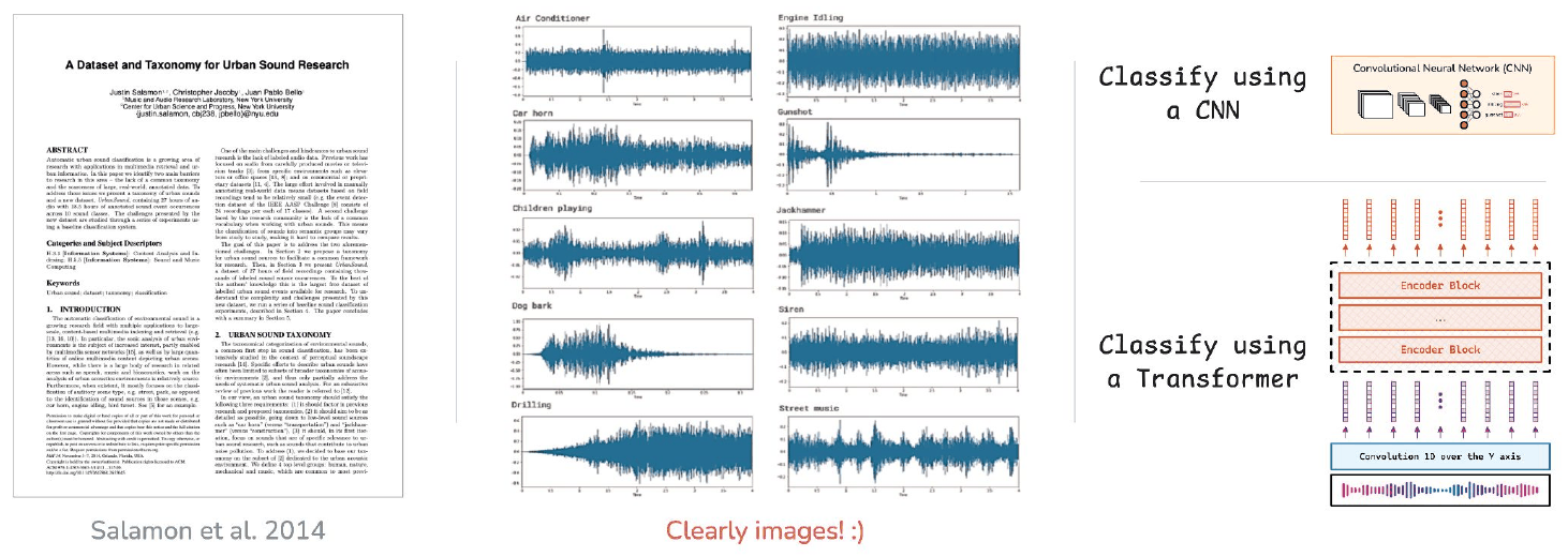
A transformer takes a sequence of vectors and does not care what the input was before it became one. Audio arrives as a waveform, sampled 16,000 times a second, which is not a sequence of vectors in any useful sense.

Two tasks.

Once audio is a spectrogram it is a two-dimensional array of intensities, so you can treat it as a picture and cut it into patches the way the vision transformer does. AST does exactly that.

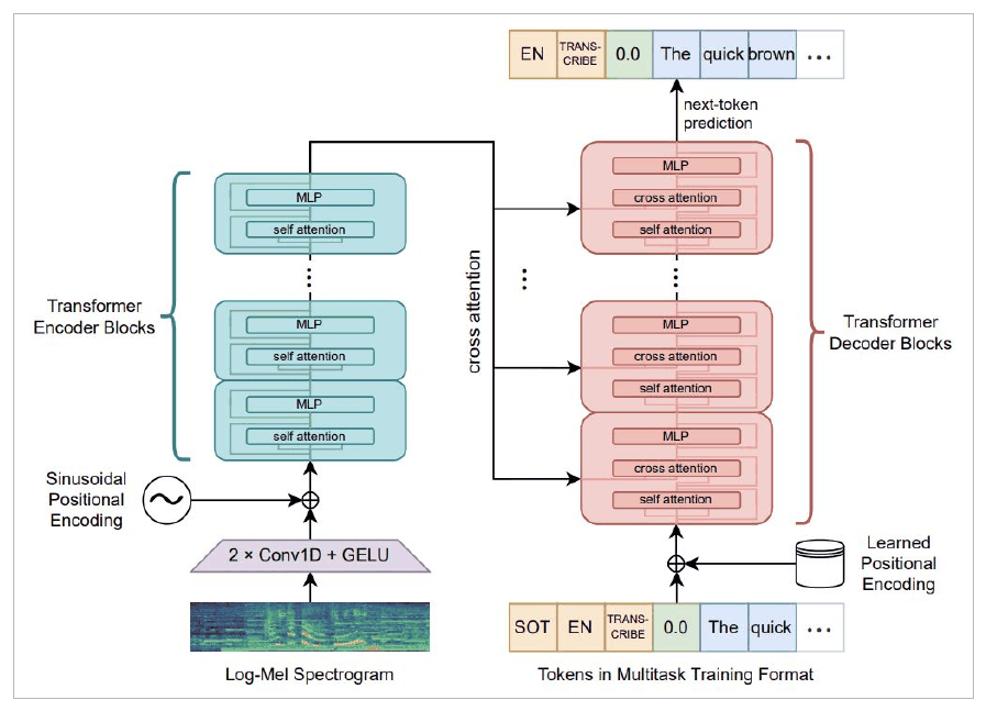
Whisper does not need to. A spectrogram is already a sequence: one column per time frame, each an 80-number vector of mel-band intensities, which is the shape a transformer wants.

The second task is the one this post follows: a speech model that has to hear a short sentence and write it down.

Log-Mel Spectrograms

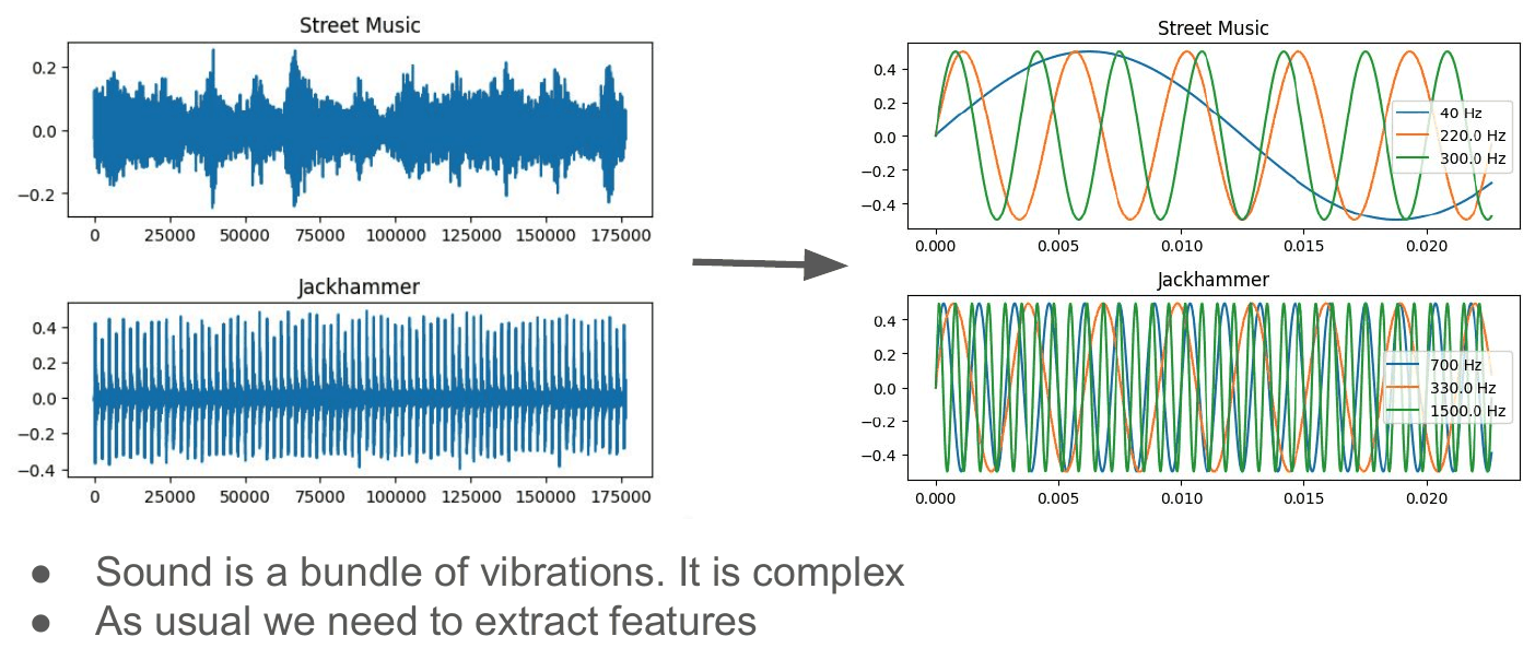
A waveform is amplitude over time, sampled 16,000 times a second, and almost none of the structure a listener cares about is visible in it directly. Two different sounds are two different bundles of vibrations at different frequencies.

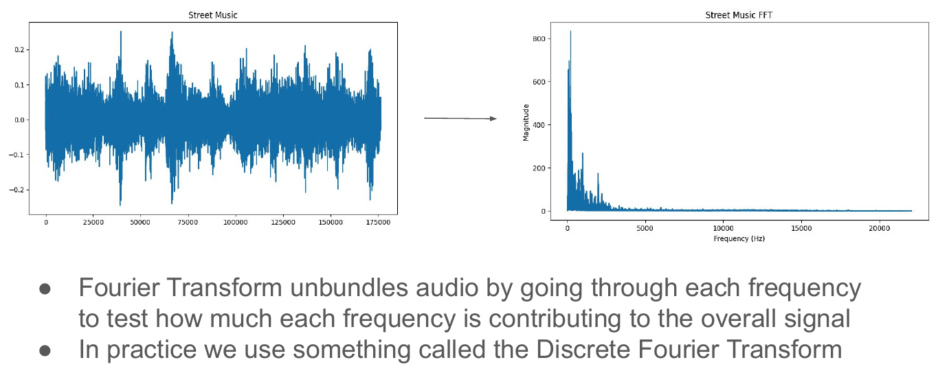
The Fourier transform unbundles it. Run it over short overlapping windows rather than the whole clip and you get frequency on one axis, time on the other, intensity as the value. That is the spectrogram, and it is why the earlier diagram could call audio “clearly images”.

Whisper adds two refinements.

• The frequency axis is squashed onto the mel scale. It spaces bands the way hearing does: fine detail low down, coarser high up. 80 bands replace 201 raw frequency bins.
• The values go through a logarithm, because loudness is perceived multiplicatively.

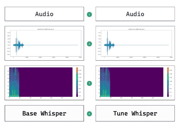
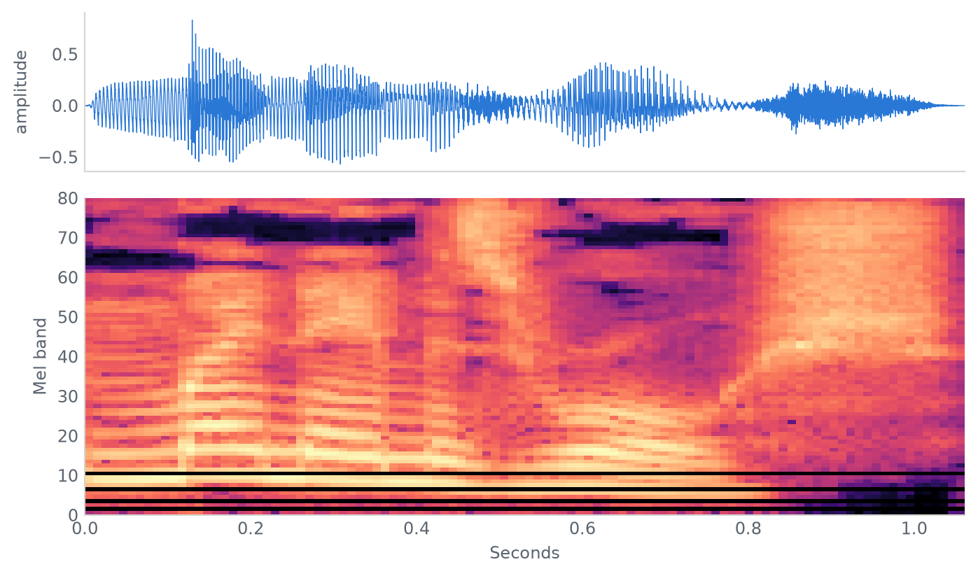
Below is that whole front end, built from scratch on the actual clip from the project, so you can see the waveform go in and the picture come out.

# Setup, inlined rather than imported so this notebook runs on its own.
# Keep it folded; nothing below it depends on anything outside this file.

import torch.nn as nn
import visualtorch
import matplotlib.pyplot as plt

# --- chart styling -------------------------------------------------------
# Categorical slots of a CVD-validated palette: blue, orange, aqua, purple.
COLOURS = ["#2a78d6", "#eb6834", "#1baf7a", "#8a63d2"]
MUTED, GRID, AXIS = "#5b6570", "#e6e6e3", "#d5d5d1"


def style_axes(ax, xlabel=None, ylabel=None, grid="y"):
    """Strip an axes back to the ink that carries information."""
    if xlabel:
        ax.set_xlabel(xlabel, color=MUTED, fontsize=9)
    if ylabel:
        ax.set_ylabel(ylabel, color=MUTED, fontsize=9)
    if grid:
        ax.grid(axis=grid, color=GRID, linewidth=0.8)
        ax.set_axisbelow(True)
    for side in ("top", "right"):
        ax.spines[side].set_visible(False)
    for side in ("left", "bottom"):
        ax.spines[side].set_color(AXIS)
    ax.tick_params(colors=MUTED, labelsize=9, length=0)
    return ax


def figure(width=7.0, height=4.2, **kw):
    fig, ax = plt.subplots(figsize=(width, height), **kw)
    return fig, ax

# --- visualtorch, configured ---------------------------------------------
# Dropout is hidden: nn.TransformerEncoderLayer exposes its internal Dropout as a
# traceable leaf, every model here builds it with dropout=0.0, and drawing a no-op
# layer says it is part of the architecture when it is not. Uncoloured it also took
# visualtorch's default orange, near enough to MultiheadAttention's to be confusing.
COLOUR_MAP = {
    nn.Linear: {"fill": COLOURS[0]},
    nn.MultiheadAttention: {"fill": COLOURS[1]},
    nn.Embedding: {"fill": COLOURS[3]},
    nn.LayerNorm: {"fill": "#aeb6bf"},
    nn.GELU: {"fill": COLOURS[2]},
    nn.ReLU: {"fill": COLOURS[2]},
    nn.Flatten: {"fill": "#aeb6bf"},
    nn.Dropout: {"fill": "#e6e6e3"},
}
_COMMON = dict(color_map=COLOUR_MAP, connector_fill="#c3c9d0", background_fill="white",
               font_color=MUTED, legend=True, show_dimension=True,
               type_ignore=[nn.Dropout])


def diagram(model, input_shape, style="graph", **overrides):
    """Render `model` as a PIL image in this site's colours.

    `graph` draws real neurons and suits a short stack; `flow` draws volumetric
    blocks whose size tracks the layer's and stays readable on a deep one. `flow`
    reports a 3-D activation as (1, 1, width), losing the sequence length, so its
    shape labels are off. `level_gap=1` keeps a residual connection drawn close to
    the blocks it skips.
    """
    if style == "graph":
        settings = dict(node_size=24, layer_spacing=110, node_spacing=8,
                        ellipsize_after=5, **_COMMON)
    else:
        settings = dict(spacing=26, scale_xy=2.4, max_xy=280, one_dim_orientation="y",
                        level_gap=1, **_COMMON)
        settings["show_dimension"] = False
    settings.update(overrides)
    return visualtorch.render(model, input_shape=input_shape, style=style, **settings)

# --- the log-mel picture -------------------------------------------------
DYNAMIC_RANGE = 8.0      # Whisper clamps the quiet end this far below the loudest


def log_mel(x, bank, n_fft, hop):
    """A waveform in, a log-mel picture out, time down the rows."""
    power = np.abs(stft(x, n_fft, hop)) ** 2
    picture = np.log10(np.maximum(bank @ power, 1e-10))
    return np.maximum(picture, picture.max() - DYNAMIC_RANGE).T.astype(np.float32)


import numpy as np
from huggingface_hub import hf_hub_download

REVISION = "f705fed08827ff6c36e3b5329495c943a5e544e8"
clip = np.load(hf_hub_download("roshbeed/ai-residency-blog-data", "audio/clip-16k.npz",
                               repo_type="dataset", revision=REVISION))
waveform, rate = clip["waveform"], int(clip["sample_rate"])

N_FFT, HOP, N_MELS = 400, 160, 80

def stft(x, n_fft, hop):
    """Fourier transform of each short overlapping window."""
    window = np.hanning(n_fft + 1)[:-1]
    frames = 1 + (len(x) - n_fft) // hop
    return np.stack([np.fft.rfft(x[i * hop:i * hop + n_fft] * window)
                     for i in range(frames)], axis=1)

def mel_filterbank(rate, n_fft, n_mels):
    """Triangular filters, evenly spaced on the mel scale rather than in hertz."""
    to_mel = lambda f: 2595 * np.log10(1 + f / 700)
    to_hz = lambda m: 700 * (10 ** (m / 2595) - 1)
    edges = to_hz(np.linspace(to_mel(0), to_mel(rate / 2), n_mels + 2))

    # The actual frequency of each FFT bin. Rounding the triangle corners to whole
    # bins instead is the tempting shortcut, and down here the mel bands are
    # narrower than one bin is wide, so several of them round onto the same corner
    # and come out empty.
    freqs = np.linspace(0, rate / 2, n_fft // 2 + 1)

    bank = np.zeros((n_mels, len(freqs)))
    for m in range(n_mels):
        left, centre, right = edges[m], edges[m + 1], edges[m + 2]
        rising = (freqs - left) / (centre - left)
        falling = (right - freqs) / (right - centre)
        bank[m] = np.maximum(0.0, np.minimum(rising, falling))
        bank[m] *= 2.0 / (right - left)     # equal area, so a wide band cannot shout
    return bank

bank = mel_filterbank(rate, N_FFT, N_MELS)
print(f"{N_MELS} filters over {bank.shape[1]} frequency bins, "
      f"{(bank.sum(1) == 0).sum()} of them empty")
spans = np.count_nonzero(bank, axis=1)
print(f"the narrowest covers {spans.min()} frequency bin, the widest {spans.max()}")

80 filters over 201 frequency bins, 0 of them empty
the narrowest covers 1 frequency bin, the widest 14

Every band carries signal, and the low ones are narrow where the high ones are wide. That spacing is what the mel scale is for. Now push the clip through them.

power = np.abs(stft(waveform, N_FFT, HOP)) ** 2
picture = np.log10(np.maximum(bank @ power, 1e-10))

# Whisper clamps the quiet end to 8 log units below the loudest point. Without it
# the floor above sets the bottom of the colour scale at -10 and every real value
# is squashed into the top of the range.
picture = np.maximum(picture, picture.max() - 8.0)

print(f"{len(waveform):,} samples at {rate} Hz = {len(waveform) / rate:.2f} seconds")
print(f"becomes an {picture.shape[0]} by {picture.shape[1]} picture, "
      f"values from {picture.min():.1f} to {picture.max():.1f}")

16,982 samples at 16000 Hz = 1.06 seconds
becomes an 80 by 104 picture, values from -6.9 to 1.1

A second of sound, 17,000 numbers long, comes out as an 80 by 104 grid. That grid is what the model reads.

Drawn, the waveform and the picture it becomes:

import matplotlib.pyplot as plt

fig, (top, bottom) = plt.subplots(2, 1, figsize=(7.4, 4.4),
                                  gridspec_kw={"height_ratios": [1, 2]})
top.plot(np.arange(len(waveform)) / rate, waveform, color=COLOURS[0], linewidth=0.5)
top.set_xlim(0, len(waveform) / rate)
style_axes(top, ylabel="amplitude", grid=None)
top.set_xticks([])
bottom.imshow(picture, aspect="auto", origin="lower", cmap="magma",
              extent=(0, len(waveform) / rate, 0, N_MELS))
style_axes(bottom, "Seconds", "Mel band", grid=None)
fig.tight_layout()

Figure 1: One second of speech, before and after. The model never sees the waveform on top.

Whisper

Structurally this is the multi-digit reader with a spectrogram where the image was.

The second of the two convolutions at the front has stride 2, halving the sequence from 3000 positions to 1500. Attention cost grows with the square of sequence length, so that one layer is a four-fold saving before any attention runs.

And a Whisper transcript does not start with words. It starts with a structured token prefix, which is how one model handles transcription, translation and language identification without being three models. For the running example that prefix is <|startoftranscript|><|en|><|transcribe|><|notimestamps|>, and the words follow it.

So the rest of this post runs Whisper. Not a model of its shape at a size that trains in seconds — the released whisper-tiny weights, on read speech, measured before and after.

import re

import torch
from transformers import WhisperForConditionalGeneration, WhisperProcessor

DEVICE = torch.device("mps" if torch.backends.mps.is_available() else "cpu")

SPEECH = "d1d9f7d1de9f83341127136398d76cce20275dd5"
data = np.load(hf_hub_download("roshbeed/ai-residency-blog-data",
                               "speech/librispeech-dummy.npz",
                               repo_type="dataset", revision=SPEECH),
               allow_pickle=True)
offsets, transcripts = data["offsets"], list(data["texts"])
samples = data["audio"]          # read out once; the .npz is lazily decompressed
clips = [samples[offsets[i]:offsets[i + 1]].astype(np.float32) / 32768.0
         for i in range(len(transcripts))]

MODEL = "openai/whisper-tiny"
processor = WhisperProcessor.from_pretrained(MODEL)
model = WhisperForConditionalGeneration.from_pretrained(MODEL).to(DEVICE)

print(f"{len(clips)} clips, {sum(map(len, clips)) / 16000:.0f} seconds of speech")
print(f"{MODEL}: {sum(p.numel() for p in model.parameters()) / 1e6:.1f}M parameters")

73 clips, 481 seconds of speech
openai/whisper-tiny: 37.8M parameters

These are the released whisper-tiny weights, and the speech is eight minutes of LibriSpeech read aloud by people the model has never heard.

Fine-tuning on One Example

The mechanism reads most easily on a clip short enough to print whole. This one is two seconds of synthesised speech saying Hello, my name is Rosh, and the released model hears the name wrong.

One Whisper detail decides whether correcting it works at all. The tokenizer puts <|startoftranscript|> at the front of a transcript, and the model prepends decoder_start_token_id itself when it shifts the labels right, and that token is start-of-transcript, so passing the tokenizer’s output through unchanged trains the decoder one position out of step. Nothing raises, the loss still falls, and the model learns a different task from the one you meant.

import copy

import librosa

SOT = processor.tokenizer.convert_tokens_to_ids("<|startoftranscript|>")


def labels_for(text):
    """Drop the tokenizer's start token; the model adds its own."""
    ids = processor.tokenizer(text, return_tensors="pt").input_ids[0]
    assert ids[0].item() == SOT, "tokenizer no longer starts with SOT"
    return ids[1:]


@torch.no_grad()
def transcription(features):
    tokens = model.generate(features, language="en", task="transcribe")
    return processor.batch_decode(tokens, skip_special_tokens=True)[0].strip()


NAME = "75ff2e33aa815ea643a2ee6513d5fa5882c58458"
spoken, _ = librosa.load(hf_hub_download("roshbeed/ai-residency-blog-data",
                                         "speech/hello-rosh.wav",
                                         repo_type="dataset", revision=NAME),
                         sr=16000)
TARGET = "Hello, my name is Rosh."
one = processor(spoken, sampling_rate=16000,
                return_tensors="pt").input_features.to(DEVICE)
one_labels = labels_for(TARGET).unsqueeze(0).to(DEVICE)

# The released weights are what everything below measures, so they go back on at
# the end. 5e-6 rather than the 1e-4 used later: eleven label tokens on two
# seconds of audio, and 1e-4 overshoots into gibberish by the second step.
released = copy.deepcopy(model.state_dict())
optimiser = torch.optim.AdamW(model.parameters(), lr=5e-6)

print(f"{len(spoken) / 16000:.2f} seconds, target {TARGET!r}\n")
print(f"{'step':>4} {'loss':>8}   transcription")
for step in range(7):
    with torch.no_grad():
        measured = model(input_features=one, labels=one_labels).loss.item()
    print(f"{step:>4} {measured:>8.4f}   {transcription(one)}")
    loss = model(input_features=one, labels=one_labels).loss
    optimiser.zero_grad()
    loss.backward()
    optimiser.step()

model.load_state_dict(released)

1.99 seconds, target 'Hello, my name is Rosh.'

step     loss   transcription

   0   4.7323   Hello, my name is Roosh.
   1   4.2688   Hello, my name is Roosh.
   2   3.9264   Hello, my name is Rosh.
   3   3.6435   Hello, my name is Rosh.
   4   3.3869   Hello, my name is Rosh.
   5   3.1449   Hello, my name is Rosh.
   6   2.9211   Hello, my name is Rosh.

<All keys matched successfully>

Two steps to move Roosh to Rosh, and the loss goes on falling after the transcript has stopped changing.

That is the whole mechanism, and on this clip it looks free. What it costs is not visible from here, which is what the rest of the post measures.

So: how good is the released model before anything is done to it. Word error rate counts substitutions, deletions and insertions against the reference, divided by the number of words in it, so 0 is perfect and 1 is as many mistakes as words.

def normalise(text):
    """LibriSpeech is uppercase and unpunctuated; Whisper is neither."""
    return re.sub(r"[^A-Z' ]", "", text.upper()).split()


def edits(reference, hypothesis):
    """Levenshtein distance over words, which is the arithmetic inside WER."""
    previous = list(range(len(hypothesis) + 1))
    for i, want in enumerate(reference, 1):
        current = [i]
        for j, got in enumerate(hypothesis, 1):
            current.append(min(previous[j] + 1, current[j - 1] + 1,
                               previous[j - 1] + (want != got)))
        previous = current
    return previous[-1]


@torch.no_grad()
def transcribe(indices, batch=16):
    out = []
    for start in range(0, len(indices), batch):
        chunk = [clips[i] for i in indices[start:start + batch]]
        features = processor(chunk, sampling_rate=16000,
                             return_tensors="pt").input_features
        tokens = model.generate(features.to(DEVICE), language="en", task="transcribe")
        out += processor.batch_decode(tokens, skip_special_tokens=True)
    return out


def word_error_rate(indices):
    errors = words = 0
    for i, hypothesis in zip(indices, transcribe(indices)):
        reference = normalise(transcripts[i])
        errors += edits(reference, normalise(hypothesis))
        words += len(reference)
    return errors / words


everything = list(range(len(clips)))
print(f"word error rate over all {len(clips)} clips: {word_error_rate(everything):.3f}")

word error rate over all 73 clips: 0.129

That is the number to keep an eye on. Everything below is measured against it.

Now find something it gets wrong. Not a contrived input — just the clip in the first dozen it handles worst.

scores = [(word_error_rate([i]), i) for i in range(12)]
worst, chosen = max(scores)

print(f"clip {chosen} is the worst of the first twelve, at {worst:.3f}")
print(f"  reference:  {transcripts[chosen]}")
print(f"  whisper:    {transcribe([chosen])[0].strip()}")

clip 4 is the worst of the first twelve, at 0.206
  reference:  LINNELL'S PICTURES ARE A SORT OF UP GUARDS AND AT EM PAINTINGS AND MASON'S EXQUISITE IDYLLS ARE AS NATIONAL AS A JINGO POEM MISTER BIRKET FOSTER'S LANDSCAPES SMILE AT ONE MUCH IN THE SAME WAY THAT MISTER CARKER USED TO FLASH HIS TEETH AND MISTER JOHN COLLIER GIVES HIS SITTER A CHEERFUL SLAP ON THE BACK BEFORE HE SAYS LIKE A SHAMPOOER IN A TURKISH BATH NEXT MAN
  whisper:    Lennils, pictures are a sort of upguards and atom paintings, and Mason's exquisite Idols are as national as a jingo poem. Mr. Birkut Foster's landscapes smile at one much in the same way that Mr. Karker used to flash his teeth. And Mr. John Colier gives his sitter a cheerful slap on the back before he says, like a shampoo or a turkish bath, next man,

A model that works, and one specific thing it gets wrong. Fine-tune on that single clip and watch two numbers: the loss on the clip, and the word error rate on clips nobody asked it to change.

Sixty-four clips are held out of every run below, rehearsal included. The eight that rehearsal draws from are kept separate from them, so the retention number is never measured on something a run has just trained on.

STEPS = 13


def batch_for(indices):
    """Features and right-padded labels; -100 keeps padding out of the loss."""
    features = processor([clips[i] for i in indices], sampling_rate=16000,
                         return_tensors="pt").input_features.to(DEVICE)
    sequences = [labels_for(transcripts[i]) for i in indices]
    labels = torch.full((len(indices), max(len(s) for s in sequences)), -100)
    for row, sequence in enumerate(sequences):
        labels[row, :len(sequence)] = sequence
    return features, labels.to(DEVICE)


others = [i for i in everything if i != chosen]
pool, held_out = others[:8], others[8:]
baseline = copy.deepcopy(model.state_dict())
target = batch_for([chosen])

print(f"fine-tune on clip {chosen}, rehearse from {len(pool)}, "
      f"measure on {len(held_out)} that no run ever trains on")


def fine_tune(rehearse, seed=0):
    """Reset to the released weights, then take STEPS on the one clip.

    `rehearse` is how many already-correct clips ride along in each batch.
    """
    model.load_state_dict(baseline)
    optimiser = torch.optim.AdamW(model.parameters(), lr=1e-4)
    generator = torch.Generator().manual_seed(seed)
    losses, clip_wer, held_wer = [], [], []

    for step in range(STEPS):
        if step:
            picked = [chosen]
            if rehearse:
                order = torch.randperm(len(pool), generator=generator)
                picked += [pool[j] for j in order[:rehearse].tolist()]
            features, labels = batch_for(picked)
            loss = model(input_features=features, labels=labels).loss
            optimiser.zero_grad()
            loss.backward()
            optimiser.step()

        # The clip's own loss either way, so the two runs plot against each other.
        with torch.no_grad():
            losses.append(model(input_features=target[0], labels=target[1]).loss.item())
        clip_wer.append(word_error_rate([chosen]))
        held_wer.append(word_error_rate(held_out))
        print(f"{step:>5} {losses[-1]:>9.4f} {clip_wer[-1]:>11.3f} "
              f"{held_wer[-1]:>14.3f}")

    return losses, clip_wer, held_wer


print(f"\n{'step':>5} {'loss':>9} {'this clip':>11} {'held out':>14}")
naive_loss, naive_clip, naive_held = fine_tune(rehearse=0)

fine-tune on clip 4, rehearse from 8, measure on 64 that no run ever trains on

 step      loss   this clip       held out
    0    1.7482       0.206          0.131
    1    0.8063       0.206          0.129
    2    0.4003       0.147          0.130
    3    0.2275       0.000          0.136
    4    0.1674       0.000          0.160
    5    0.1491       0.118          0.185
    6    0.1386       0.044          0.194
    7    0.1309       0.044          0.233
    8    0.1257       0.044          0.286
    9    0.1213       0.044          0.690
   10    0.1168       0.044          0.705
   11    0.1121       0.044          0.955
   12    0.1075       0.044          0.925

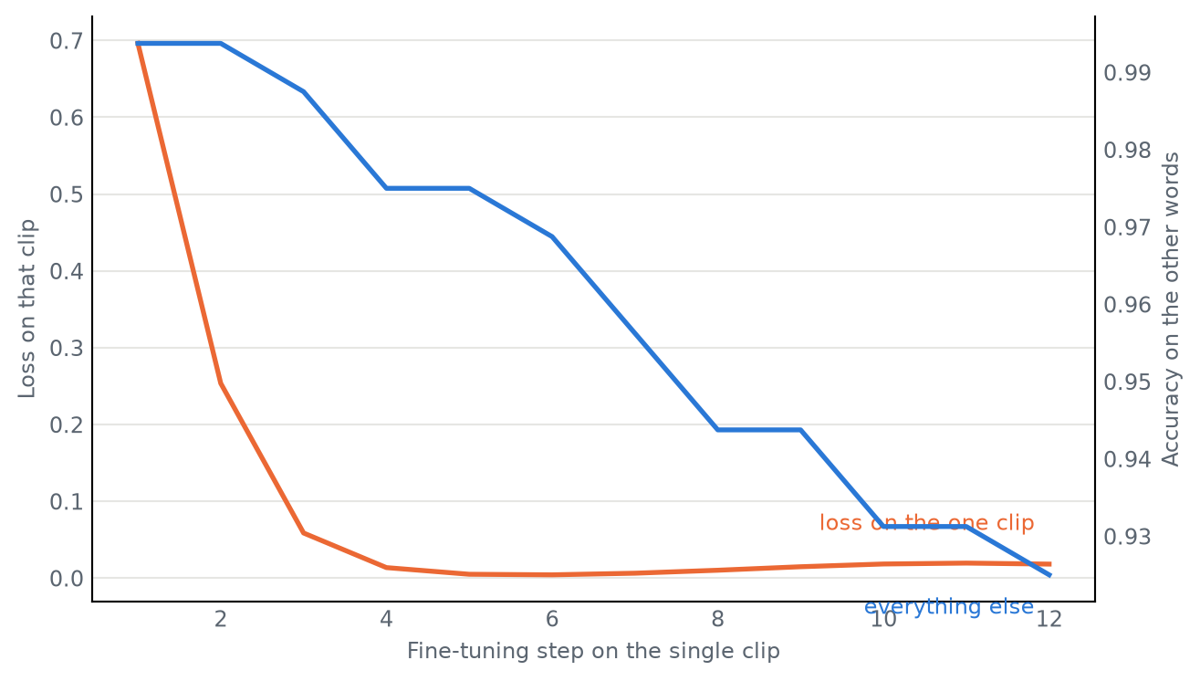
Three steps and the clip is transcribed exactly right. Nothing after that improves it. The clip sits at 0.044 from step six onward while the loss crawls from 0.149 to 0.108, which is the model memorising a transcript it already gets right.

The right-hand column is what those steps cost. Word error rate on the sixty-four held-out clips goes 0.136, 0.194, 0.690, 0.925. The model ends barely able to transcribe speech it handled fine twelve steps earlier, and the loss being optimised fell the whole way.

Both numbers on one chart, the clip’s loss against the held-out set’s error rate:

import matplotlib.pyplot as plt

fig, ax = figure(height=4.0)
ax.plot(range(STEPS), naive_loss, color=COLOURS[1], linewidth=2)
style_axes(ax, "Fine-tuning step on the single clip", "Loss on that clip")
ax.annotate("loss on the clip", xy=(STEPS - 1, naive_loss[-1]), xytext=(-6, 10),
            textcoords="offset points", ha="right", fontsize=9, color=COLOURS[1])

right = ax.twinx()
right.plot(range(STEPS), naive_held, color=COLOURS[0], linewidth=2)
right.set_ylabel("Word error rate, the held_out clips", color=MUTED, fontsize=9)
right.tick_params(colors=MUTED, labelsize=9, length=0)
for side in ("top", "left"):
    right.spines[side].set_visible(False)
right.spines["right"].set_color(AXIS)
right.annotate("everything else", xy=(STEPS - 1, naive_held[-1]), xytext=(-6, -14),
               textcoords="offset points", ha="right", fontsize=9, color=COLOURS[0])
fig.tight_layout()

Figure 2: The fix lands within a few steps. Everything after that is the model memorising one clip at the expense of the clips it was never asked to change.

Catastrophic Forgetting

A few gradient steps correct the clip, and the loss on it falls to nearly zero.

With one training example, a loss near zero means the model has memorised that clip rather than learned anything that carries, which is what goes wrong when the same procedure is scaled up.

Word error rate on the held-out clips goes from 0.131 to 0.925 over those same thirteen steps, from a working transcriber to one that gets most words wrong, while the only number the loop prints is falling. Training hard on one narrow task overwrites what the model could already do, which is catastrophic forgetting, and nothing inside the fine-tuning loop reports it.

Rehearsal

Nothing in that loop constrains the other clips. The only gradient comes from one example, so that example is the only term in the objective and the rest of the function is unconstrained.

Rehearsal puts the old task back in the batch. Alongside the clip being fixed, each step carries a few clips the model already handles, drawn from a pool held aside for it. Their loss is already low, so they contribute almost no gradient until a step starts to raise it.

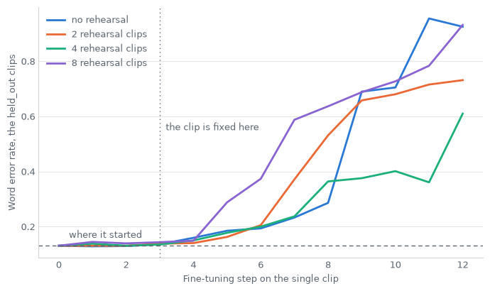
The cost is having kept some of the original data. Same clip, same learning rate, same thirteen steps, varying only how many clips ride along.

rehearsed = {}
for size in (2, 4, 8):
    print(f"--- {size} rehearsal clips per step")
    print(f"{'step':>5} {'loss':>9} {'this clip':>11} {'held out':>14}")
    rehearsed[size] = fine_tune(rehearse=size)

print(f"\nheld-out clips, {STEPS - 1} steps in, from {naive_held[0]:.3f}")
print(f"  no rehearsal   {naive_held[-1]:.3f}   "
      f"clip {naive_clip[-1]:.3f}")
for size, (_, clip_wer, held_out) in rehearsed.items():
    print(f"  {size} clips       {held_out[-1]:.3f}   clip {clip_wer[-1]:.3f}")

best = min(rehearsed, key=lambda s: rehearsed[s][2][-1])
print(f"\nbest rehearsal size here is {best}, at {rehearsed[best][2][-1]:.3f} "
      f"against {naive_held[-1]:.3f} without")
print(f"every run's lowest held-out error is still its first few steps: "
      f"{min(naive_held):.3f}")

--- 2 rehearsal clips per step
 step      loss   this clip       held out
    0    1.7482       0.206          0.131
    1    0.8341       0.250          0.131
    2    0.3875       0.059          0.131
    3    0.2257       0.015          0.138
    4    0.1685       0.000          0.141
    5    0.1488       0.044          0.163
    6    0.1381       0.044          0.206
    7    0.1308       0.044          0.372
    8    0.1240       0.985          0.531
    9    0.1179       0.985          0.658
   10    0.1127       0.985          0.681
   11    0.1101       0.985          0.716
   12    0.1066       0.044          0.732
--- 4 rehearsal clips per step
 step      loss   this clip       held out
    0    1.7482       0.206          0.131
    1    0.8909       0.221          0.138
    2    0.3737       0.044          0.131
    3    0.2474       0.029          0.135
    4    0.1869       0.000          0.150
    5    0.1572       0.000          0.178
    6    0.1431       0.000          0.200
    7    0.1337       0.000          0.237
    8    0.1264       0.000          0.364
    9    0.1203       0.000          0.376
   10    0.1147       0.000          0.401
   11    0.1094       0.000          0.361
   12    0.1051       0.000          0.610
--- 8 rehearsal clips per step
 step      loss   this clip       held out
    0    1.7482       0.206          0.131
    1    0.9323       0.221          0.145
    2    0.4186       0.118          0.140
    3    0.2643       0.029          0.144
    4    0.1919       0.000          0.149
    5    0.1584       0.015          0.289
    6    0.1417       0.985          0.374
    7    0.1299       0.985          0.588
    8    0.1204       0.985          0.637
    9    0.1128       0.985          0.688
   10    0.1065       0.985          0.727
   11    0.1008       0.985          0.784
   12    0.0956       0.985          0.932

held-out clips, 12 steps in, from 0.131
  no rehearsal   0.925   clip 0.044
  2 clips       0.732   clip 0.044
  4 clips       0.610   clip 0.000
  8 clips       0.932   clip 0.985

best rehearsal size here is 4, at 0.610 against 0.925 without
every run's lowest held-out error is still its first few steps: 0.129

fig, ax = figure(height=4.2)
curves = [(0, naive_held)] + [(s, r[2]) for s, r in rehearsed.items()]
for (size, held_out), colour in zip(curves, COLOURS):
    ax.plot(range(STEPS), held_out, color=colour, linewidth=2,
            label=f"{size} rehearsal clips" if size else "no rehearsal")
ax.axhline(naive_held[0], color=MUTED, linewidth=1, linestyle=(0, (4, 3)))
ax.axvline(3, color=MUTED, linewidth=1, linestyle=(0, (1, 3)))
style_axes(ax, "Fine-tuning step on the single clip",
           "Word error rate, the held_out clips")
ax.annotate("where it started", xy=(0.3, naive_held[0]), xytext=(0, 8),
            textcoords="offset points", fontsize=9, color=MUTED)
ax.annotate("the clip is fixed here", xy=(3, 0.55), xytext=(6, 0),
            textcoords="offset points", fontsize=9, color=MUTED)
legend = ax.legend(frameon=False, fontsize=9, loc="upper left")
for text in legend.get_texts():
    text.set_color(MUTED)
fig.tight_layout()

Figure 3: The same clip, the same learning rate, the same thirteen steps. Rehearsal slows the damage and does not stop it; the flat part at the left is the only place the model is both fixed and intact.

Rehearsal reduces the damage without removing it.

Four clips per step is the best of the sizes tried, ending at 0.610 against 0.925 with none, and the clip itself reaches 0.000 rather than 0.044. Two clips land between them at 0.732. Eight is worse than doing nothing at all, at 0.932, with the target clip broken as well at 0.985, though that is one seed and the clip being fixed is only an eighth of each batch there.

Every curve on that chart still ends far above where it started.

The lowest held-out error any run reaches is 0.129, and the clip is already perfect at step three without rehearsal and step four with it, while the held-out set is still at 0.136 and 0.150. That two-or-three-step window is where the model has learned the thing you wanted without having paid for it yet.

The window is invisible from inside the training loop. The loss on the clip falls smoothly through it and keeps falling afterwards, the same shape on both sides of the cliff. The only signal comes from the sixty-four clips nobody is training on, and only if you spend the compute to measure them.

Conclusion

• A spectrogram is already a sequence of frames, so the transformer machinery applies to it
• Whisper is an encoder-decoder over that sequence
• Fine-tuning on one example works, and works fast
• It also costs you accuracy everywhere else, and nothing reports that
• Rehearsal slows that cost and does not remove it
• There is a two-or-three-step window where the fix has landed and the damage has not, and stopping inside it is the technique
• You can only see that window from the data you are not training on

The full project is on GitHub.