RLHF with PPO from Scratch: Four Models, GAE and LoRA
rl
rlhf
language
The reference, the policy, the reward model and the value model, and the arithmetic that turns one score for a finished summary into a gradient per token.
Author
Rosh Beed
Published
July 13, 2026
Preference optimisation.
Most tasks have a loss function sitting there waiting. Predict the missing word. Predict the digit. Predict the next character. This one starts from a task where there’s no such thing.
Write down the loss for a good summary. You cannot. There’s no target string to compare against, and two perfectly good summaries share almost no tokens.
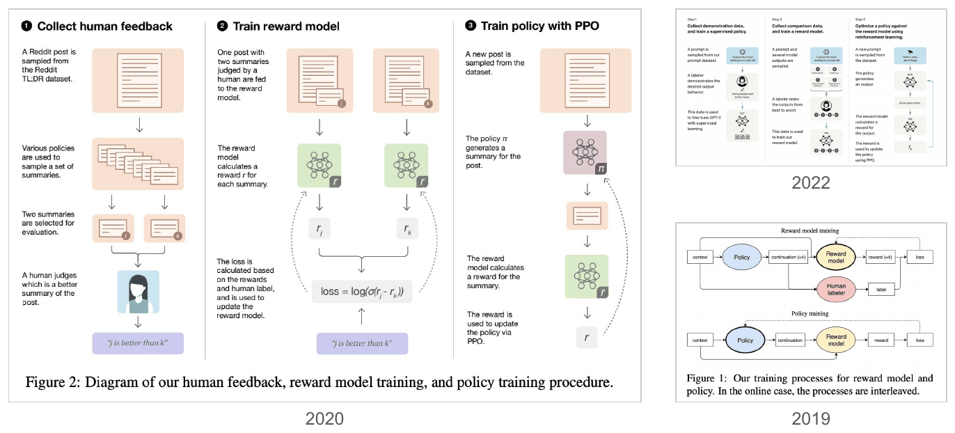
What you can do is show a person two summaries and ask which they prefer, which is how Stiennon et al. trained a summariser on this same Reddit data. That’s cheap and reliable, and it gives you comparisons rather than targets.
Three stages, and this implements the third: optimising the language model against a reward model that was itself fitted to human comparisons.
Which means the thing being maximised is itself a model, wrong in places nobody has looked. The sweep at the end measures whether that goes wrong here.
The PPO Loop, Step by Step
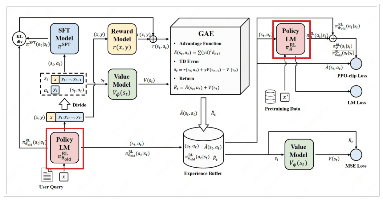
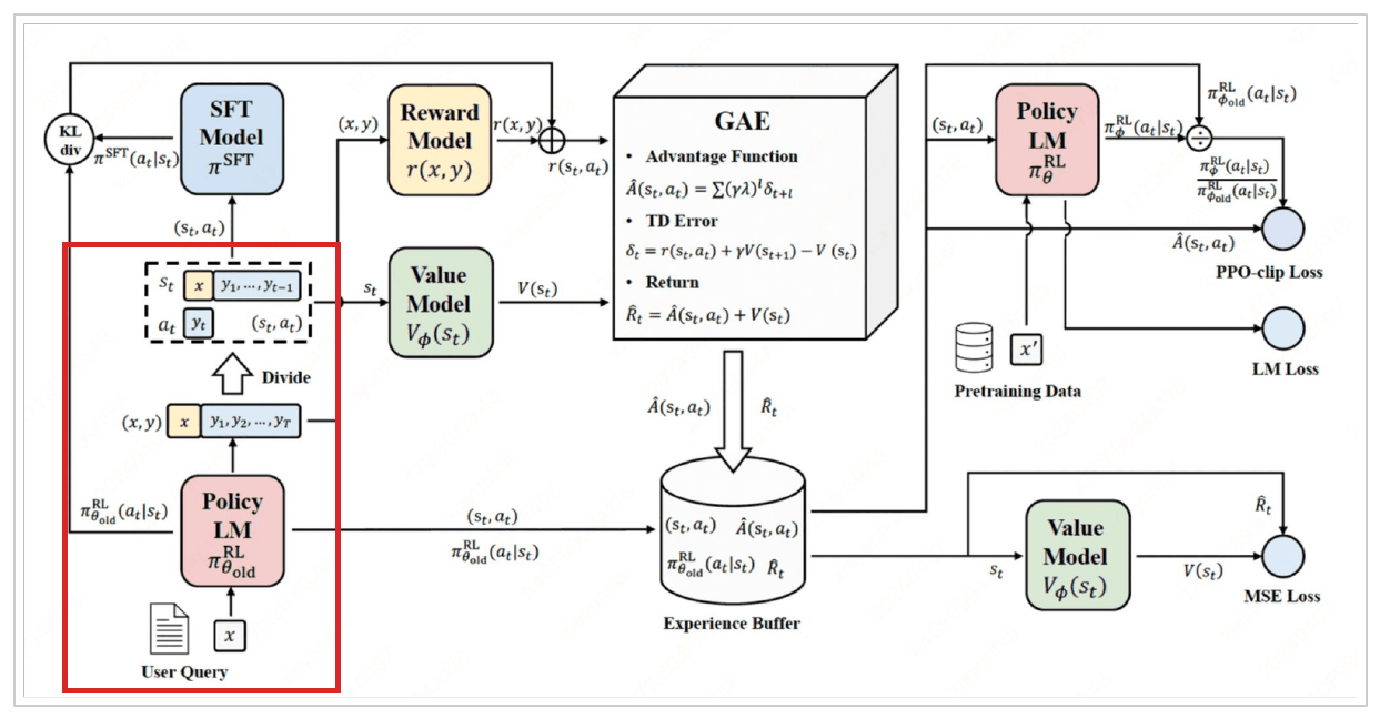
Four models, an advantage calculation and a buffer. Before any of that makes sense, the shape underneath it does.
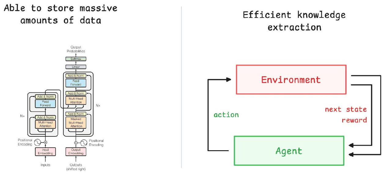
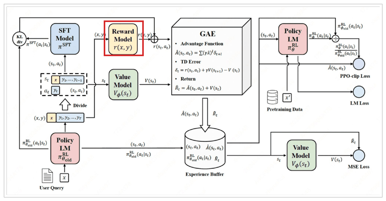
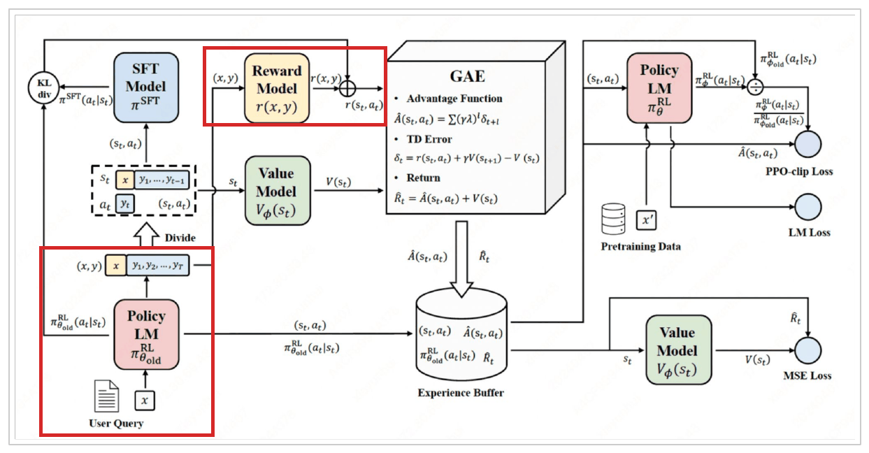
Generating a summary is an episode. The policy picks a token, that changes the state, and at the end the reward model scores what came out.
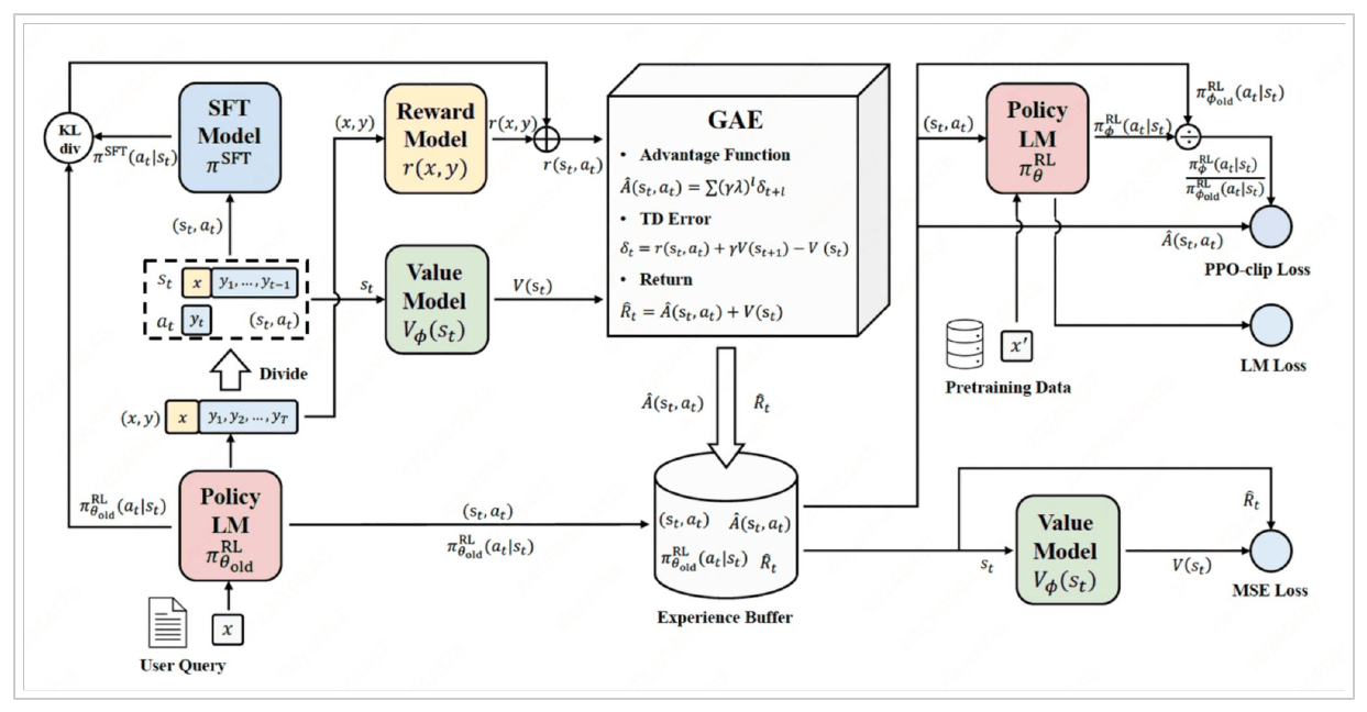
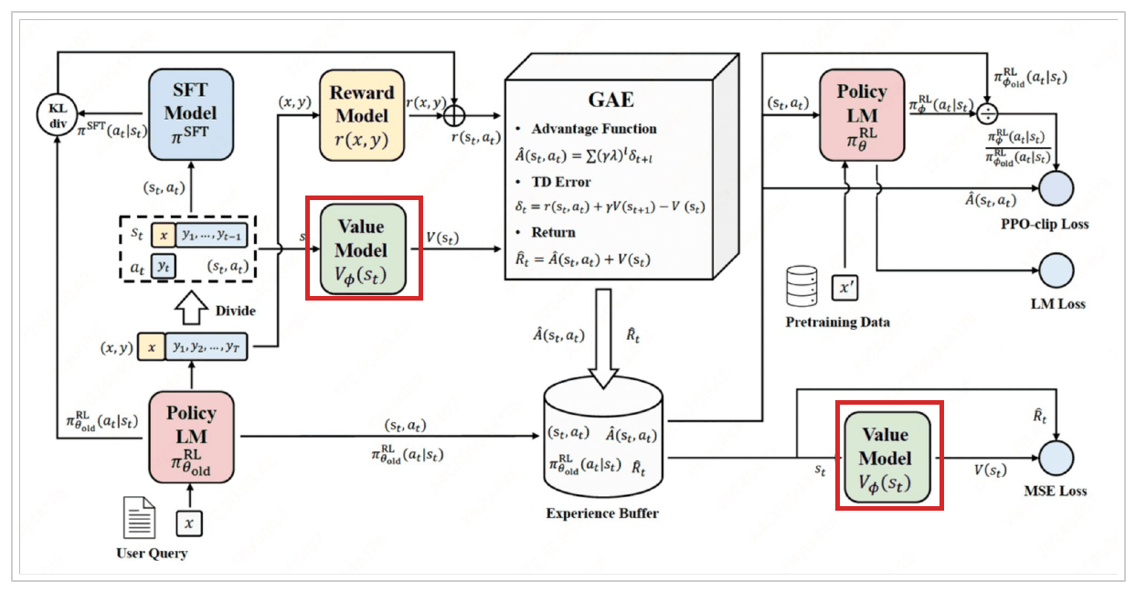
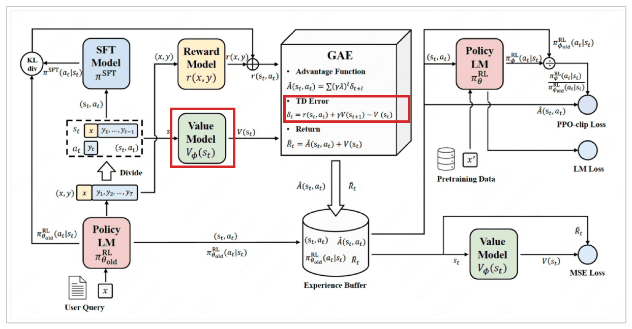
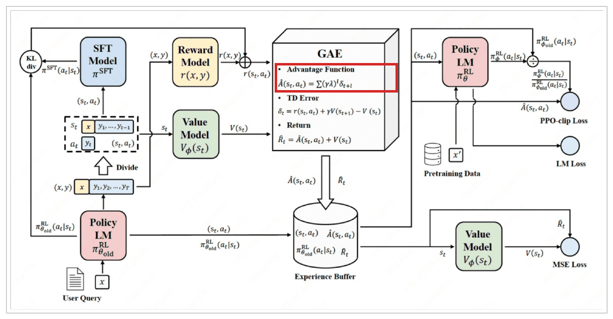
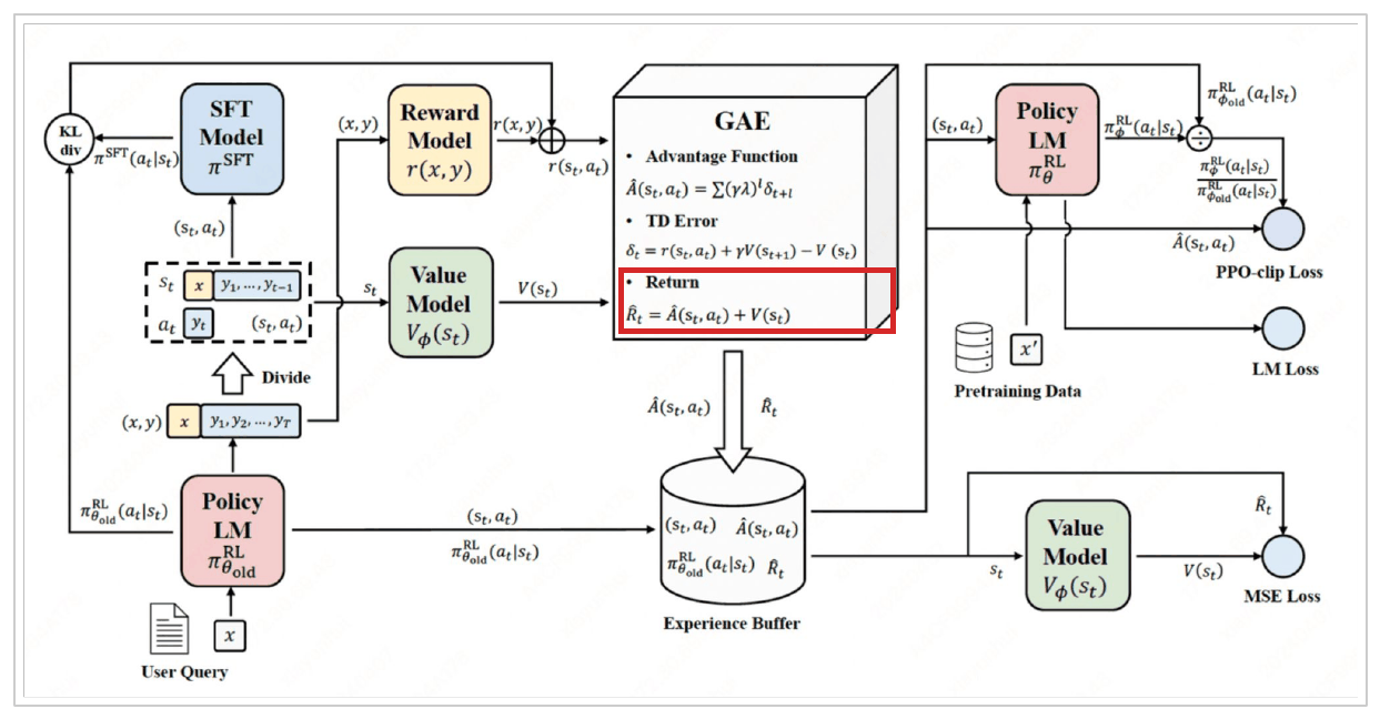
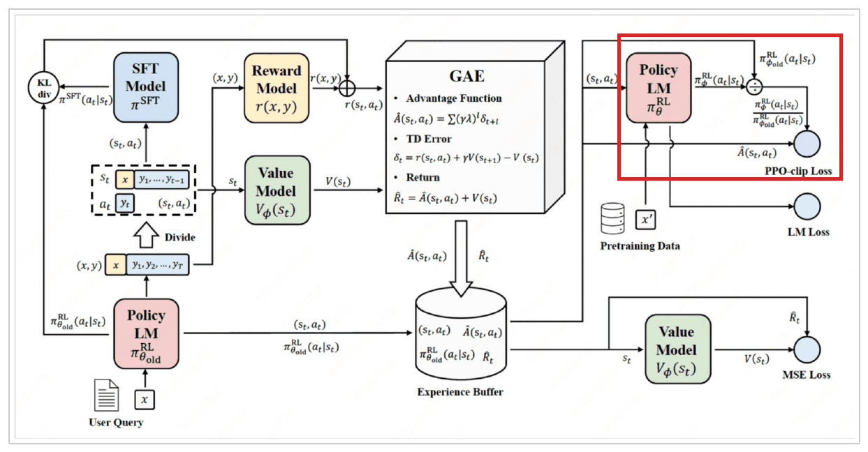
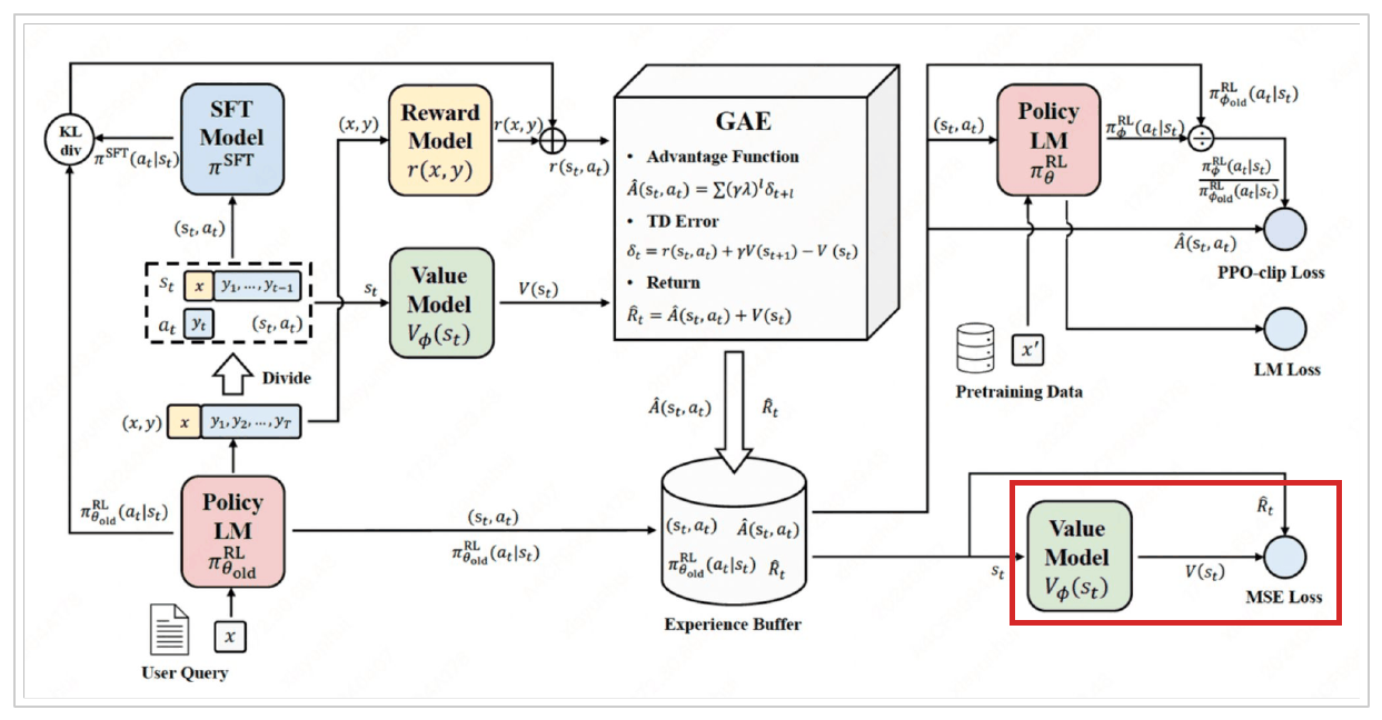
One score, for the whole summary. The optimiser needs a number for every token in it. Everything else in the overview diagram exists to get from the first to the second, and the rest of this section walks it one box at a time.
The four models
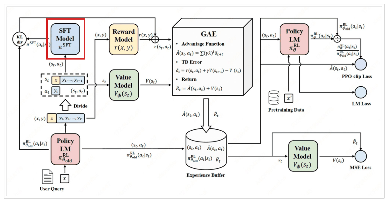
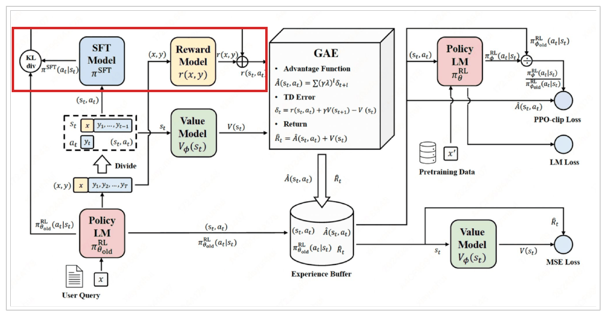
The reference. The SFT model, frozen for the whole run. It supplies the log-probability of the generated text under the model we started from, and the KL penalty measures drift against that.
The policy. The same model with a small trainable adapter on top. That adapter is the only tensor here that receives a gradient.
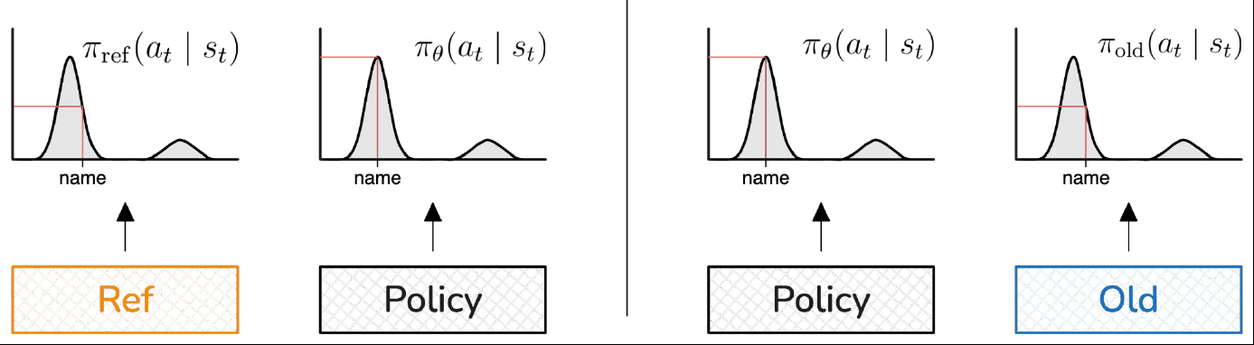
It appears twice in the diagram because PPO needs both versions at once: the old policy that generated the batch, and the current one being updated. Clipping acts on the ratio between them, which is what makes it safe to take several gradient steps on a single batch.
The reward model. Reads a post and a summary of it, returns one number. It is the only source of quality signal in the loop, and an approximation of the preferences it was fitted to rather than those preferences themselves.
The value model. A linear head on the policy’s last hidden state, predicting what each position is worth. It trains alongside the policy and is thrown away at the end.
It also appears twice, for a different reason. It computes the advantage, and is then regressed onto the return that advantage helped produce.
Loading them, then. The reference and the reward model are frozen from here, and only a copy of the reference is ever updated.
Show the code
import copyimport numpy as npimport torchimport torch.nn.functional as Ffrom datasets import load_datasetfrom torch import nnfrom transformers import (AutoModelForCausalLM, AutoModelForSequenceClassification, AutoTokenizer)DEVICE = torch.device("mps"if torch.backends.mps.is_available() else"cpu")POLICY_NAME ="HuggingFaceTB/SmolLM2-135M-Instruct"REWARD_NAME ="OpenAssistant/reward-model-deberta-v3-large-v2"TLDR, TLDR_REVISION ="trl-lib/tldr", "21233da376667088e6eb1ce4ce19ed832c2935d3"MAX_NEW_TOKENS, TEMPERATURE, TOP_K, TOP_P =48, 1.0, 50, 0.95PROMPT_TOKENS, BATCH =256, 16tokeniser = AutoTokenizer.from_pretrained(POLICY_NAME)reference = AutoModelForCausalLM.from_pretrained( POLICY_NAME, dtype=torch.float32).to(DEVICE).eval()reward_tokeniser = AutoTokenizer.from_pretrained(REWARD_NAME)reward_model = AutoModelForSequenceClassification.from_pretrained( REWARD_NAME).to(DEVICE).eval()for parameter in (*reference.parameters(), *reward_model.parameters()): parameter.requires_grad =False# Reddit posts, each already ending in "TL;DR:", beside the summary a person wrote.# Short ones only, so a batch of sixteen fits alongside four models.tldr = load_dataset(TLDR, split="train[:2000]", revision=TLDR_REVISION)short = [r for r in tldr iflen(tokeniser(r["prompt"]).input_ids) <= PROMPT_TOKENS]PROMPTS = [r["prompt"] for r in short[:BATCH]]HUMAN = [r["completion"].strip() for r in short[:BATCH]]print(f"policy {sum(p.numel() for p in reference.parameters()) /1e6:>6.0f}M")print(f"reward {sum(p.numel() for p in reward_model.parameters()) /1e6:>6.0f}M")print(f"{len(PROMPTS)} posts, up to {MAX_NEW_TOKENS} tokens of summary each\n")print(PROMPTS[0][:400])print(f"\nthe summary a person wrote: {HUMAN[0]!r}")
policy       135M
reward       435M
16 posts, up to 48 tokens of summary each

SUBREDDIT: r/relationships

TITLE: Is it weird that this turned me off from my gf?

POST: The other day my girlfriend(23 years old) and myself(22 years old) were talking and she revealed to me that she almost didn't date me because I was too short (5'7"-5'8").  She is only about 5'5".  Now she loves me a lot and thinks I am the best thing to ever happen to her but for some reason, learning about t

the summary a person wrote: "Gf said she almost didn't date me because I was too short.  Now I am really turned off by her."
That copy is what gets the adapter. Every attention projection keeps its frozen base weight and gains a thin trainable update beside it, initialised so the update starts as a no-op and the wrapped model begins identical to the reference.
Show the code
LORA_R, LORA_ALPHA =16, 32class LoRALinear(nn.Module):"""A frozen Linear with a trainable low-rank update beside it."""def__init__(self, base, rank=LORA_R, alpha=LORA_ALPHA):super().__init__()self.base = basefor parameter inself.base.parameters(): parameter.requires_grad =Falseself.down = nn.Linear(base.in_features, rank, bias=False)self.up = nn.Linear(rank, base.out_features, bias=False) nn.init.normal_(self.down.weight, std=0.01) nn.init.zeros_(self.up.weight) # so the adapter starts as a no-opself.scale = alpha / rankdef forward(self, x):returnself.base(x) +self.up(self.down(x)) *self.scaledef with_lora(model):"""Wrap every attention projection; leave everything else alone."""for layer in model.model.layers: attention = layer.self_attnfor name in ("q_proj", "v_proj"):setattr(attention, name, LoRALinear(getattr(attention, name)).to(DEVICE))return modelexample = with_lora(copy.deepcopy(reference))trainable =sum(p.numel() for p in example.parameters() if p.requires_grad)print(f"{trainable:,} trainable of "f"{sum(p.numel() for p in example.parameters()):,} "f"({trainable /sum(p.numel() for p in example.parameters()):.2%})")del example
921,600 trainable of 135,436,608 (0.68%)
Generating and scoring
An iteration starts by rolling out an episode: sample a summary for each post, then score the pair.
Token ids carry the whole way through. A generated summary is never decoded to text and re-encoded to score it, because decode-then-encode is not a round trip and the two sides of the ratio would end up scoring different sequences.
Show the code
encoded = tokeniser(PROMPTS, return_tensors="pt", padding=True, padding_side="left").to(DEVICE)PROMPT_LEN = encoded["input_ids"].shape[1]@torch.no_grad()def generate(model, generator):"""Sample a summary per post, keeping the ids that were sampled.""" out = model.generate(**encoded, max_new_tokens=MAX_NEW_TOKENS, do_sample=True, top_k=TOP_K, top_p=TOP_P, temperature=TEMPERATURE, pad_token_id=tokeniser.pad_token_id or tokeniser.eos_token_id)return out, out[:, PROMPT_LEN:]def token_log_probs(model, sequences, actions):"""log p(action | everything before it), for the ids actually sampled.""" logits = model(sequences).logits[:, PROMPT_LEN -1:-1]return torch.log_softmax(logits, -1).gather(-1, actions.unsqueeze(-1)).squeeze(-1)@torch.no_grad()def score_summaries(summaries):"""The reward model's score for each post and summary pair.""" pairs = reward_tokeniser(PROMPTS, summaries, return_tensors="pt", padding=True, truncation=True).to(DEVICE)return reward_model(**pairs).logits.squeeze(-1)@torch.no_grad()def score(actions): summaries = tokeniser.batch_decode(actions, skip_special_tokens=True)return score_summaries(summaries), summaries@torch.no_grad()def fluency(sequences, actions):"""The reference model's total log-probability of the summary."""return token_log_probs(reference, sequences, actions).sum(-1)generator = torch.Generator(device=DEVICE).manual_seed(0)sequences, actions = generate(reference, generator)rewards, summaries = score(actions)print(f"reference: reward {rewards.mean():.2f}, "f"fluency {fluency(sequences, actions).mean():.1f}")print(f"the human TL;DRs score {score_summaries(HUMAN).mean():.2f}\n")for summary in summaries[:2]:print(f" {summary.strip()[:110]!r}")
reference: reward -4.81, fluency -109.3
the human TL;DRs score 3.55

  "Is my friend a typical middle-aged woman who doesn't have a lot to say and is a total jerk?\n\nEDIT: I just got "
  'I listen to the song and am wondering if I am numb (that was on my top list). Could you help me?\n\nEDIT: I got '
That is the floor: an untrained summariser, and what the reward model makes of it. The summaries a person wrote are the other end of the range. Every number later in this post sits between the two.
The state and the action
\[
s_t = (x,\, y_{1:t-1})
\tag{1}\]
\[
a_t = y_t
\tag{2}\]
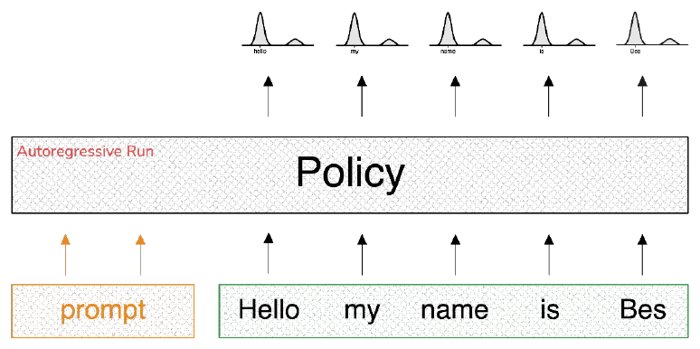
A state is the prompt plus everything written so far; the action is the next token. One forty-eight-token summary is forty-eight state–action pairs, not one training example.
One forward pass over the generated sequences yields both \(\log \pi_\theta(a_t \mid s_t)\) and \(V_\phi(s_t)\): a log-probability and a value for every generated token. Offsetting the logits by one position lines each prediction up with the token it predicts.
Show the code
CLIP, INNER_STEPS, LR, VALUE_LR =0.2, 2, 1e-4, 1e-4GAMMA, LAM, ITERATIONS =0.99, 0.95, 100class ValueHead(nn.Module):"""The fourth model. One scalar per state: what this position is worth."""def__init__(self, width):super().__init__()self.project = nn.Linear(width, 1)def forward(self, hidden):returnself.project(hidden).squeeze(-1)def policy_forward(policy, value_head, sequences, actions):"""Log-probs and values for the same positions, from one forward pass. in: sequences (B, prompt+T), actions (B, T) out: log pi(a_t | s_t) and V(s_t), both (B, T) """ out = policy(sequences, output_hidden_states=True) logits = out.logits[:, PROMPT_LEN -1:-1] chosen = torch.log_softmax(logits, -1).gather(-1, actions.unsqueeze(-1)).squeeze(-1) hidden = out.hidden_states[-1][:, PROMPT_LEN -1:-1]return chosen, value_head(hidden)
The KL term applies at every position, because the policy can drift at any of them. The score lands on the final token alone, because that is the only point at which there is a finished summary to score.
The KL is estimated from log-probs that already exist rather than by comparing full distributions: the difference of the two models’ log-probabilities at the token actually taken.
That looks like the clipped ratio, which is also a difference of log-probs. The second model is what separates them. This one compares the policy against the frozen reference, which never moves all run; the ratio compares the policy against itself a few gradient steps ago.
This is reward shaping, not a term in the loss. The penalty goes through the advantage so it is discounted and credited like any other reward. Put it in the loss directly, differentiable, and the sign works against you.
Show the code
def shaped_rewards(old, base, rewards, kl_coefficient):"""Per-token reward: a KL penalty everywhere, the score at the last token. in: old and base log-probs (B, T), sequence rewards (B,) out: r_t, (B, T) The reward model reads the whole generation and returns one number, so it lands on the final token. The KL term is per token because the policy can drift at any of them. """ shaped =-kl_coefficient * (old - base) shaped[:, -1] = shaped[:, -1] + rewardsreturn shaped
GAE accumulates those backwards, discounted by \(\gamma\lambda\), so a token’s advantage carries the errors that follow it as well as its own. That is how a score arriving only at the last token reaches the tokens that earned it.
\[
\hat{R}_t = \hat{A}_t + V_\phi(s_t)
\tag{7}\]
Reward-to-go, which is the value model’s regression target. A single backwards pass over the sequence produces the advantage and this target together.
Show the code
def advantages_and_returns(per_token, values):"""TD errors, then GAE, then reward-to-go. in: r_t and V(s_t), both (B, T) out: the advantage estimate and the value target, both (B, T) delta_t = r_t + gamma V(s_t+1) - V(s_t) asks whether this token did better than the value model expected. GAE accumulates those backwards, discounted by gamma*lam, so an advantage carries the errors after it as well as its own. """ steps = per_token.shape[1] advantages = torch.zeros_like(per_token) running = torch.zeros_like(per_token[:, 0])for t inreversed(range(steps)): following = values[:, t +1] if t +1< steps else torch.zeros_like(values[:, 0]) delta = per_token[:, t] + GAMMA * following - values[:, t] running = delta + GAMMA * LAM * running advantages[:, t] = runningreturn advantages, advantages + values # reward-to-go
Two things have to hold for that. The adapter has to start as a no-op, so the policy begins identical to the reference. And the forward pass used in training has to line up with the one used in generation, slice for slice, so both score the same token at the same position.
Get either wrong and the ratio is not 1 before a single gradient step. Clipping then acts on a value that never started at the centre of its range, and nothing raises.
Show the code
# The policy the inner loop starts from: a copy of the reference with the adapter# attached. Its log-probs go through the training path, the reference's through the# generation path, and the two have to agree before any gradient step.probe = with_lora(copy.deepcopy(reference))probe_head = ValueHead(reference.config.hidden_size).to(DEVICE)with torch.no_grad(): old = token_log_probs(reference, sequences, actions) new, _ = policy_forward(probe, probe_head, sequences, actions)ratio = (new - old).exp()print(f"ratio at the first inner step: {ratio.min():.4f} to {ratio.max():.4f}")print(f"clip range: {1- CLIP:.1f} to {1+ CLIP:.1f}")del probe, probe_head
ratio at the first inner step: 1.0000 to 1.0000
clip range: 0.8 to 1.2
The adapter is a no-op and the two paths agree, so the ratio is 1 and clipping stays inert until the policy actually moves.
Taking the smaller of the clipped and unclipped terms, which is PPO’s contribution, stops a single batch moving the policy a long way. Several gradient steps on one batch of generations is why PPO is cheaper than regenerating every time, and the clip is what makes that safe.
\[
\mathrm{clip}(x, a, b) = \begin{cases}
a, & x < a \\
x, & a \le x \le b \\
b, & x > b
\end{cases}
\]
Once the policy has moved far enough on a sample, that sample contributes no further gradient.
Clipping and the KL penalty are different constraints. Clipping bounds how far one update moves the policy from the policy that collected the batch. The KL penalty bounds how far the whole run moves it from the model you started with.
You can clip perfectly and still walk somewhere useless, one small safe step at a time.
Plain MSE against the reward-to-go. It is added to the policy loss, so one backward pass trains both, with separate learning rates in the optimiser’s two groups.
The rest of the objective
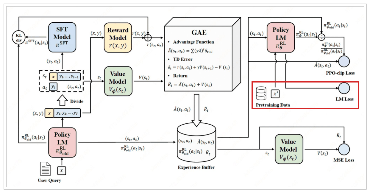
Two more terms appear in the full statement. One of them is a box in the diagram that nothing so far has accounted for.
An entropy bonus. Maximising entropy keeps the policy’s distribution spread out, which is the standard guard in RL against collapsing onto one phrasing that scores well and never exploring past it.
Ordinary next-token likelihood on pretraining data, mixed into the same update. That is the boxed region: a store of pretraining text, a batch drawn from it, and the LM loss it feeds. InstructGPT adds this term so that chasing the reward does not cost the model its general language ability, which is the same failure the KL penalty guards against, reached from the other side.
The four terms with their coefficients. The run below sets \(c_v = 1\) and the other two to zero, so the loss it computes is the first two terms of this.
Show the code
def ppo_losses(new, old, advantage, predicted, target):"""The clipped policy objective and the value regression, as one number. in: new and old log-probs (B, T), the advantage (B, T), the value model's prediction and its target (B, T) out: the scalar to call backward on, and the value loss on its own The min of the clipped and unclipped terms is what stops one batch moving the policy a long way, which is what makes it safe to take several steps on it. """ ratio = (new - old).exp() clipped = torch.min(ratio * advantage, ratio.clamp(1- CLIP, 1+ CLIP) * advantage) value_loss = F.mse_loss(predicted, target)return-clipped.sum(-1).mean() + value_loss, value_loss
Putting it together
One iteration generates a batch of summaries, scores them, works out the advantages once with no gradient flowing, and then takes a few clipped steps on that same batch. A hundred iterations to a run.
The coefficient \(\beta\) on the KL penalty is the only thing that changes between runs: five values, three seeds each.
baseline_reward =float(rewards.mean())baseline_fluency =float(fluency(sequences, actions).mean())print(f"{'KL':>6}{'reward, worst to best':>24}{'fluency':>20}{'value loss':>12}")for coefficient, runs in results.items(): got =sorted(r for r, _, _, _ in runs) flu =sorted(f for _, f, _, _ in runs) val = np.mean([v for _, _, v, _ in runs])print(f"{coefficient:>6}{got[0]:>10.2f} to {got[-1]:>9.2f} "f"{flu[0]:>9.1f} to {flu[-1]:>8.1f}{val:>12.3f}")print(f"{'(ref)':>6}{baseline_reward:>10.2f}{'':>13}{baseline_fluency:>9.1f}")middle =sorted(results[0.5], key=lambda r: r[0])[len(SEEDS) //2]print(f"\nat KL 0.5, a median answer: {middle[3][0][:60]!r}")
    KL    reward, worst to best              fluency   value loss
   0.0      -4.46 to     -3.16    -107.2 to    -87.0        1.535
  0.01      -4.65 to     -3.43    -100.6 to    -94.8        3.231
   0.1      -4.59 to     -4.11    -109.3 to    -69.0       10.529
   0.5      -4.84 to     -4.34    -116.0 to    -96.9        1.570
   2.0      -4.99 to     -4.20    -117.0 to    -99.8        1.824
 (ref)      -4.81                 -109.3

at KL 0.5, a median answer: " I'm not turning into a woman to do something I don't care a"
Every coefficient’s best seed beats the reference on reward. The worst seeds at \(\beta = 0.5\) and \(\beta = 2.0\) do not, ending at −4.84 and −4.99 against the reference’s −4.81.
The penalty costs reward here, it does not buy it.
The best run of the sweep is at \(\beta = 0\), reaching −3.16 with no penalty at all, and the reward falls as the coefficient rises. That is the textbook trade working as advertised: the penalty is paid in reward to stay close to the model you started from.
Fluency does not pay it back. At \(\beta = 0\) the summaries score −107.2 to −87.0 against the reference’s −109.3, so the unpenalised runs are no less ordinary under the reference than the penalised ones. On this task, over a hundred iterations, the KL term is not demonstrably earning its place.
The spread is the finding.
Three seeds, same code, same data, same coefficient, and \(\beta = 0\) alone runs from −4.46 to −3.16. That range is as wide as the gap between most of the coefficients, so the ordering between adjacent settings is not something three seeds can settle.
Any single run would support whatever conclusion it happened to land on, which is why the table reports the worst and the best rather than a mean.
The value loss sits near 1.5 at most settings and jumps to 10.5 at \(\beta = 0.1\), which is one run’s critic failing to track a moving target rather than anything about that coefficient.
None of it gets close to a person. The summaries people wrote score 3.55 against the policy’s best of −3.16, so the whole sweep moves about a fifth of the distance from the untrained model to the human reference. A 135M policy, a hundred iterations and a small adapter is not the configuration that closes that gap.
A reward model that can be saturated, some phrase that scores full marks whatever the prompt, is the failure RLHF is usually warned about. A preference model trained on human comparisons is harder to corner than a rule, and the summaries stayed English at every coefficient.
Two Ways the Ratio Stops Starting at 1
Score token ids, never re-tokenized text. Recording a generated state as its decoded string and re-encoding it looks equivalent and is not. About one state in twenty does not survive decode-then-encode, sometimes coming back with a different number of tokens, and the two sides of the ratio then score different sequences.
Sum the log-ratios. A sequence ratio is the exponential of the summed log-ratios. Summing the per-token ratios instead gives the sequence length: six here, against a clip range of 0.8 to 1.2.
Clipping is then engaged from the first step of every iteration, which quietly means positive advantages contribute no gradient and the policy only ever learns from its failures. Nothing errors and the loss still falls.
The check above is two lines and catches both.
Conclusion
A reward model turns preferences into a number, and that number is the only supervision there is
The reward is one scalar for a finished summary; every other quantity in the loop is per token
Shaping puts the KL penalty at every position and the score at the last one, so both reach the policy through the same advantage
GAE spreads credit backwards, which is how a score arriving at the end reaches the tokens that earned it
The value model supplies the baseline the advantage is measured against, and is trained against the return it helped compute
Clipping bounds how far one update moves from the policy that collected the batch; the KL penalty bounds how far training moves from the model you started with
The clip is what makes a batch safe to reuse for several steps, and reuse is what makes PPO cheaper than regenerating every time