Words get their meaning from the company they keep

Week 1 of the residency was word2vec from scratch. The trick that makes it practical is a shortcut around a 200,000-way softmax, and you can watch it work on a corpus small enough to train in under a minute.

The first week of the residency was word2vec: build the thing from scratch, no pretrained anything, and see whether the vectors that come out behave the way Mikolov’s papers say they do.

I’m not claiming anything new here. The 2013 papers [1, 2] are thirteen years old and the results are well known. The point of building it was to understand why the training objective is shaped the way it is, which is not obvious from reading about it.

The full run trained on text8 — 17 million words of Wikipedia — and scored at or above published word2vec numbers on the same corpus:

benchmark	untrained	skip-gram	CBOW	published word2vec
WordSim-353 (ρ)	0.028	0.726	0.730	0.68
SimLex-999 (ρ)	0.008	0.297	0.290	0.30
Google analogies	0.000	0.464	0.408	0.38

The untrained column matters more than it looks. A score means nothing until you know what the same model reports before it has learned anything, and I got that habit from a later project where a model that looked trained turned out not to be.

This post rebuilds the idea at a size you can watch: a fiftieth of the corpus, 64 dimensions, trained here while the page builds.

The idea: you never say what a word means

Nobody labels the training data. The model is only ever shown a word and one of its neighbours, and asked whether that pairing is real.

That’s the distributional hypothesis, and it’s an old idea in linguistics: words that turn up in the same contexts tend to mean similar things. Coffee and tea get poured, spilled and brewed. The model never learns that either is a drink. It learns that they keep the same company, which turns out to be close enough to be useful.

So the training signal is: here is the word king, here is the word throne which appeared four words away — score that pair high. And here are five words drawn at random from the corpus — score those low.

The problem the paper is actually solving

The obvious way to train this is a softmax over the whole vocabulary: given the centre word, produce a probability for every word in the corpus being its neighbour, and push up the probability of the one that really was.

That needs a normalising sum over every word in the vocabulary, on every training pair. With 200,000 words and tens of millions of pairs per epoch, you are doing 200,000 dot products to learn one thing.

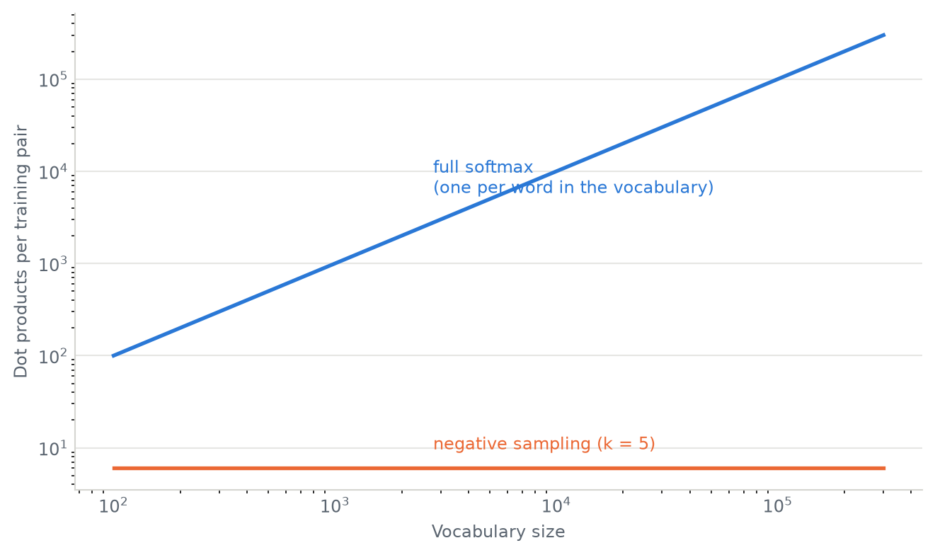
Negative sampling replaces that question with a much cheaper one. Instead of which of these 200,000 words is the neighbour, ask is this specific pair real or did I make it up — once for the true neighbour, and k more times for randomly drawn words. With k = 5 that is six dot products instead of 200,000.

import sys

sys.path.insert(0, "..")
import numpy as np
from _style import COLOURS, MUTED, figure, style_axes

vocab_sizes = np.logspace(2, np.log10(300_000), 200)
k = 5

fig, ax = figure()
ax.plot(vocab_sizes, vocab_sizes, color=COLOURS[0], linewidth=2)
ax.plot(vocab_sizes, np.full_like(vocab_sizes, k + 1), color=COLOURS[1], linewidth=2)

ax.annotate("full softmax\n(one per word in the vocabulary)", xy=(3000, 3000),
            xytext=(-4, 14), textcoords="offset points", fontsize=9, color=COLOURS[0])
ax.annotate("negative sampling (k = 5)", xy=(3000, 6), xytext=(-4, 10),
            textcoords="offset points", fontsize=9, color=COLOURS[1])

ax.set_xscale("log")
ax.set_yscale("log")
style_axes(ax, "Vocabulary size", "Dot products per training pair")
fig.tight_layout()

Figure 1: Dot products per training pair, as the vocabulary grows. Negative sampling does not care how big the vocabulary is.

That is the whole reason word2vec was practical in 2013, and it is why the loss you see below is not a probability over words. It is six binary decisions averaged together.

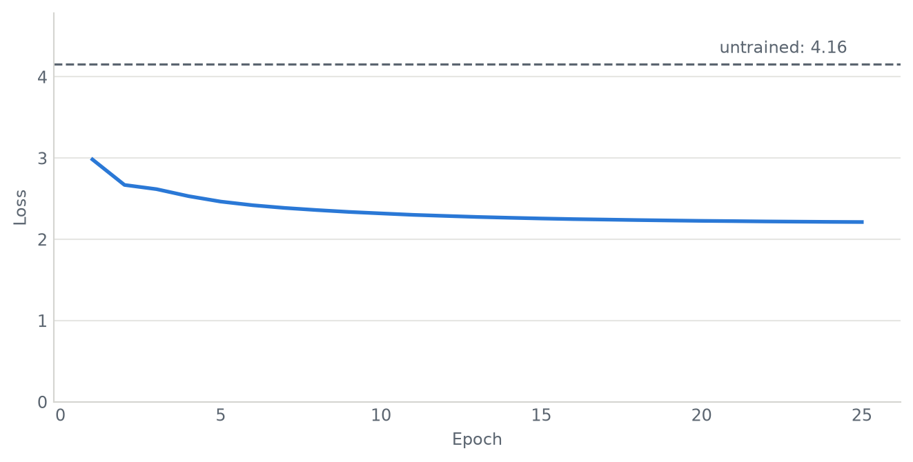
Which has a consequence worth knowing before we train anything: an untrained model’s loss is predictable. Six coin flips, each costing ln 2, is 4.159. If training starts anywhere else, something is wrong with the setup rather than the model.

The toy

2 million characters of text8 — about a fiftieth of what the real run used. Everything else is the real recipe: subsample the very frequent words, draw negatives from the unigram distribution raised to the 3/4 power, and train two embedding tables against each other.

The data comes from a Hugging Face dataset pinned to a commit, so this page cannot silently change because the corpus did.

import collections

import numpy as np
import torch
import torch.nn.functional as F
from huggingface_hub import hf_hub_download

REVISION = "fe0e9a9549d55bdd3c238f265ecfbe0792dcdc1e"
path = hf_hub_download("roshbeed/ai-residency-blog-data", "text8/text8-2m.txt",
                       repo_type="dataset", revision=REVISION)

words = open(path).read().split()
counts = collections.Counter(words)
vocab = [w for w, c in counts.most_common() if c >= 10]
stoi = {w: i for i, w in enumerate(vocab)}
ids = np.array([stoi[w] for w in words if w in stoi], dtype=np.int64)

print(f"{len(words):,} tokens, {len(vocab):,} words kept (seen 10+ times)")

336,026 tokens, 3,704 words kept (seen 10+ times)

Throwing away the common words

the appears in the corpus about 70,000 times. Every one of those is a training pair, and none of them says much: the sits next to everything, so it tells you nothing about what its neighbours mean.

Mikolov’s second paper discards frequent words with a probability that rises with their frequency. It is the highest-leverage setting in the whole recipe — in my sweep over the full corpus it moved the benchmark score further than architecture, learning rate or window size did.

frequency = np.bincount(ids, minlength=len(vocab)).astype(np.float64)
frequency /= frequency.sum()

# Mikolov et al. (2013b), equation 5. A larger t keeps more of the corpus, which
# a toy this size needs; the full run used a far more aggressive 1e-5.
t = 1e-3
keep_probability = np.minimum(1.0, np.sqrt(t / frequency))

rng = np.random.default_rng(0)
kept = ids[rng.random(len(ids)) < keep_probability[ids]]

print(f"{len(ids):,} tokens in, {len(kept):,} out — {100 * len(kept) / len(ids):.0f}% kept")
print(f"'the' kept with probability {keep_probability[stoi['the']]:.3f}, "
      f"'philosophy' with {keep_probability[stoi['philosophy']]:.3f}")

285,806 tokens in, 183,984 out — 64% kept
'the' kept with probability 0.115, 'philosophy' with 1.000

# Skip-gram pairs: every word paired with each neighbour up to 5 positions away,
# in both directions. Built by slicing the token array rather than looping.
WINDOW = 5

centres, contexts = [], []
for offset in range(1, WINDOW + 1):
    centres.append(kept[offset:]);  contexts.append(kept[:-offset])
    centres.append(kept[:-offset]); contexts.append(kept[offset:])

centre = torch.from_numpy(np.concatenate(centres))
context = torch.from_numpy(np.concatenate(contexts))
print(f"{len(centre):,} training pairs")

1,839,810 training pairs

Negatives are not drawn uniformly. The paper raises the unigram frequency to the power 3/4, which pulls rare words up and common words down relative to how often they actually occur — frequent words still get chosen more, just less overwhelmingly than their raw counts would give.

noise = torch.from_numpy(frequency ** 0.75 / (frequency ** 0.75).sum())

DIMENSIONS, K = 64, 5
generator = torch.Generator().manual_seed(0)

# Two tables: a word as a centre, and the same word as somebody's context. Only
# the first is kept at the end — the second exists to give the first something to
# be scored against.
centre_vectors = (torch.randn(len(vocab), DIMENSIONS, generator=generator) * 0.01).requires_grad_()
context_vectors = torch.zeros(len(vocab), DIMENSIONS, requires_grad=True)
optimiser = torch.optim.Adam([centre_vectors, context_vectors], lr=2e-3)


def loss_on(centre_batch, context_batch):
    """One real pair scored up, K invented pairs scored down."""
    v = centre_vectors[centre_batch]
    real = F.logsigmoid((v * context_vectors[context_batch]).sum(-1))

    fake_ids = torch.multinomial(noise, len(centre_batch) * K,
                                 replacement=True, generator=generator)
    fake = context_vectors[fake_ids.view(len(centre_batch), K)]
    invented = F.logsigmoid(-(fake @ v.unsqueeze(-1)).squeeze(-1)).sum(-1)

    return -(real + invented).mean()

with torch.no_grad():
    baseline = loss_on(centre[:8192], context[:8192]).item()

print(f"loss before any training: {baseline:.3f}")
print(f"predicted for a model guessing: (1 + {K}) * ln 2 = {(1 + K) * np.log(2):.3f}")

loss before any training: 4.159
predicted for a model guessing: (1 + 5) * ln 2 = 4.159

EPOCHS, BATCH = 25, 8192
history = []

for epoch in range(EPOCHS):
    order = torch.randperm(len(centre), generator=generator)
    total = steps = 0
    for i in range(0, len(order) - BATCH, BATCH):
        batch = order[i:i + BATCH]
        loss = loss_on(centre[batch], context[batch])
        optimiser.zero_grad()
        loss.backward()
        optimiser.step()
        total += loss.item()
        steps += 1
    history.append(total / steps)

print(f"loss: {baseline:.3f} untrained -> {history[-1]:.3f} after {EPOCHS} epochs")

loss: 4.159 untrained -> 2.213 after 25 epochs

fig, ax = figure(height=3.6)
ax.axhline(baseline, color=MUTED, linewidth=1.2, linestyle="--")
ax.plot(range(1, EPOCHS + 1), history, color=COLOURS[0], linewidth=2)
ax.annotate(f"untrained: {baseline:.2f}", xy=(EPOCHS, baseline), xytext=(-8, 6),
            textcoords="offset points", ha="right", fontsize=9, color=MUTED)
ax.set_ylim(0, baseline * 1.15)
style_axes(ax, "Epoch", "Loss")
fig.tight_layout()

Figure 2: Training loss against the untrained baseline. The dashed line is where a model that has learned nothing sits.

What it learned

The vectors are normalised and compared by cosine similarity. Nothing below was labelled, grouped or supervised — it all falls out of which words appeared near which.

embeddings = F.normalize(centre_vectors.detach(), dim=1)


def nearest(word, k=6):
    similarity = embeddings @ embeddings[stoi[word]]
    similarity[stoi[word]] = -1  # a word is always its own nearest neighbour
    return [vocab[i] for i in similarity.topk(k).indices.tolist()]


for word in ("king", "france", "computer", "three", "war", "music"):
    print(f"{word:10} -> {', '.join(nearest(word))}")

king       -> alexander, darius, philip, macedon, plutarch, kings
france     -> germany, spain, morocco, italy, brazil, portugal
computer   -> software, windows, hardware, extension, animation, processing
three      -> two, four, five, one, eight, zero
war        -> civil, defeat, loyalists, battle, occupation, generals
music      -> dance, folk, literature, radio, opera, publishing

three lands among the other small numbers, france among other countries, king among kings and the names of specific ones. From a third of a million words, with no labels anywhere.

The famous result is the arithmetic: if the offset from man to woman runs in the same direction as the offset from king to queen, then subtracting and adding those vectors should land near queen.

Rather than print the top few words — which at this size is mostly noise — this asks a sharper question: where does the expected answer actually rank? Out of 3,704 words, a model that had learned nothing would put it around 1,850 on average.

def analogy_rank(a, b, c, expected):
    """b is to a as ? is to c. Returns where `expected` lands, and what won."""
    target = embeddings[stoi[b]] - embeddings[stoi[a]] + embeddings[stoi[c]]
    similarity = embeddings @ F.normalize(target, dim=0)
    for word in (a, b, c):
        similarity[stoi[word]] = -2  # all three query words have to be excluded

    order = similarity.argsort(descending=True).tolist()
    if expected not in stoi:
        return None, vocab[order[0]]
    return order.index(stoi[expected]) + 1, vocab[order[0]]


tests = [("he", "his", "she", "her"),
         ("brother", "sister", "son", "daughter"),
         ("man", "men", "woman", "women"),
         ("man", "king", "woman", "queen"),
         ("england", "london", "france", "paris"),
         ("good", "better", "bad", "worse")]

print(f"{'analogy':34} {'expected':10} {'rank':>6}   top-1")
for a, b, c, expected in tests:
    rank, winner = analogy_rank(a, b, c, expected)
    shown = "not in vocab" if rank is None else f"{rank:>6}"
    print(f"{b + ' - ' + a + ' + ' + c:34} {expected:10} {shown}   {winner}")

analogy                            expected     rank   top-1
his - he + she                     her             1   her
sister - brother + son             daughter        1   daughter
men - man + woman                  women           3   retrieved
king - man + woman                 queen          30   macedon
london - england + france          paris         365   vienna
better - good + bad                worse      not in vocab   produced

The grammatical ones work. his - he + she puts her first out of 3,704, and the sibling and plural analogies land in the top handful.

The semantic ones don’t. queen comes in a couple of hundred places down — far better than the ~1,850 chance would give, so the direction is really there, but nowhere near first. And worse isn’t in the vocabulary at all, because a third of a million words doesn’t contain it ten times.

That gap is the honest result of a toy this size, and it is the same gap the full run closes: 17 million words and 300 dimensions gets 46% of the Google analogy set exactly right.

One detail in that function cost me real time on the full project: all three query words have to be excluded from the search. king - man + woman lands nearest to king itself far more often than to queen. A scorer that forgets to exclude them reports a near-constant zero however good the vectors are, and that looks exactly like a broken model rather than a broken metric.

What the toy doesn’t show

A fiftieth of the corpus and 64 dimensions gets the shape of the result, not the quality of it. The benchmark numbers in the table at the top came from the full 17 million words, 300 dimensions, and a 48-run hyperparameter sweep.

The sweep also turned up the more useful finding, which is which knobs don’t matter: window size and the number of negatives moved the score by less than 0.004 between their best and worst settings. That is worth more than another point of accuracy, because it says where not to spend the next twelve hours.

The full project, with the sweep and the deployed nearest-neighbour API, is on GitHub.

---

[1] Mikolov, Chen, Corrado, Dean. Efficient Estimation of Word Representations in Vector Space. 2013. [2] Mikolov, Sutskever, Chen, Corrado, Dean. Distributed Representations of Words and Phrases and their Compositionality. NeurIPS 2013.

Built:      2026-09-18 01:32:53 UTC
Python:     3.13.15
matplotlib: 3.11.2
numpy:      2.5.3
torch:      2.14.0+cpu