I asked a sweep how many dimensions I needed, and it refused to answer

A 48-run Bayesian hyperparameter search over six knobs, one of which was embedding size. It found a good model and told me almost nothing about the question I actually had.

When I trained word2vec from scratch, one of the settings I had to pick was how many numbers each word vector gets. 100? 300? The papers use 300 and so does nearly everyone, but I wanted to know what it was buying.

So I did what seemed obvious: put embedding size into the hyperparameter sweep along with everything else. 48 runs, twelve hours, Bayesian search over architecture, embedding size, window, negatives, subsampling and learning rate, ranked on a composite of three word-similarity benchmarks.

It found a good configuration. It could not answer my question, and the reason is worth more than the answer was.

import json
import sys

sys.path.insert(0, "..")
import numpy as np
from _style import COLOURS, MUTED, figure, style_axes

runs = json.load(open("sweep-runs.json"))
print(f"{len(runs)} completed runs")

sizes, counts = np.unique([r["embed_size"] for r in runs], return_counts=True)
for size, count in zip(sizes, counts):
    print(f"  {size:>3} dimensions: {count:>2} runs {'#' * count}")

48 completed runs
  100 dimensions:  1 runs #
  200 dimensions:  4 runs ####
  300 dimensions: 43 runs ###########################################

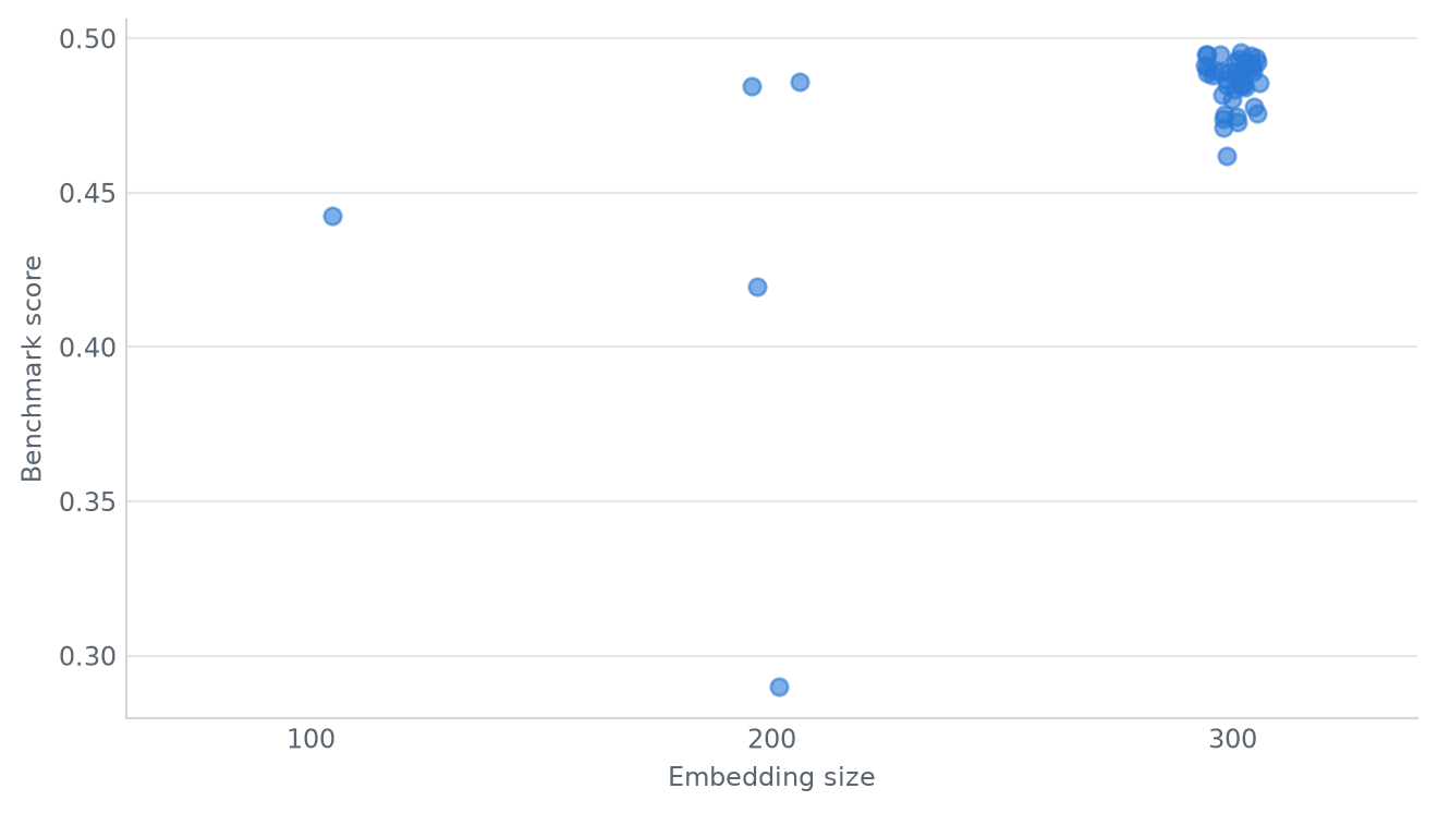
There it is. Of 48 runs, 43 chose 300 dimensions. One run — one — tried 100.

That isn’t a bug. It is Bayesian optimisation doing exactly its job. It builds a model of which settings score well and spends the remaining budget there. Early on it found that 300 dimensions and skip-gram were working, and from then on it mostly stopped looking anywhere else.

Which is what you want if the question is what is the best model I can find in twelve hours. It is precisely wrong if the question is what does this one knob do, because the answer to the second question lives in the settings the search deliberately abandons.

fig, ax = figure(height=4.0)
jitter = np.random.default_rng(0).uniform(-6, 6, len(runs))
ax.scatter([r["embed_size"] for r in runs] + jitter, [r["score"] for r in runs],
           s=34, color=COLOURS[0], alpha=0.6, zorder=3)

ax.set_xticks([100, 200, 300])
ax.set_xlim(60, 340)
style_axes(ax, "Embedding size", "Benchmark score")
fig.tight_layout()

Figure 1: Every run in the sweep, by embedding size. The 300-dimension column is the search exploiting; the other two columns are almost empty, so they carry almost no information.

Reading a trend off that would be self-deception. The 300 column has 43 runs spanning 0.46 to 0.50, which is a wider spread than any gap between the columns — so the variation within one setting swamps the difference between settings. And the 100-dimension point is a single run that also differed in window size and learning rate, so whatever it shows isn’t attributable to dimensions.

One accidental exception

Digging through the runs, the search did produce one genuinely controlled comparison, by luck rather than design.

def matches(a, b, keys=("architecture", "window_size", "num_negatives", "subsample_threshold")):
    return all(a[k] == b[k] for k in keys)


pairs = [(a, b) for a in runs for b in runs
         if a["embed_size"] > b["embed_size"] and matches(a, b)
         and abs(a["learning_rate"] - b["learning_rate"]) / a["learning_rate"] < 0.02]

for a, b in pairs:
    print(f"{a['architecture']}, window {a['window_size']}, {a['num_negatives']} negatives, "
          f"subsample {a['subsample_threshold']:g}")
    print(f"  learning rate {a['learning_rate']:.5f} vs {b['learning_rate']:.5f}")
    print(f"  {a['embed_size']} dimensions: {a['score']:.4f}")
    print(f"  {b['embed_size']} dimensions: {b['score']:.4f}")
    print(f"  difference: {a['score'] - b['score']:+.4f}")

skipgram, window 8, 10 negatives, subsample 1e-05
  learning rate 0.00215 vs 0.00214
  300 dimensions: 0.4956
  200 dimensions: 0.4860
  difference: +0.0096

Two runs identical in architecture, window, negatives and subsampling, with learning rates within 0.5% of each other, differing only in embedding size. The extra 100 dimensions are worth about 0.01 on the benchmark.

That’s one data point, from a search that was not trying to produce it. It’s suggestive and it is not a curve.

Just run the experiment

The thing I should have done from the start, and it turns out to be cheap: hold everything else fixed and vary the one setting. Five runs, not forty-eight.

Here it is on the small corpus from the word2vec post — a fiftieth of the data the real sweep used, so the numbers are lower throughout, but the shape is the point. Scored against WordSim-353, where humans rated how related pairs of words are and the model is judged on whether it agrees.

import collections
import re

import torch
import torch.nn.functional as F
from huggingface_hub import hf_hub_download

DATASET, REVISION = "roshbeed/ai-residency-blog-data", "9113ea48905b4f7178b333919ed5ec1a474561d7"

words = open(hf_hub_download(DATASET, "text8/text8-2m.txt",
                             repo_type="dataset", revision=REVISION)).read().split()
counts = collections.Counter(words)
vocabulary = [w for w, c in counts.most_common() if c >= 10]
index = {w: i for i, w in enumerate(vocabulary)}
ids = np.array([index[w] for w in words if w in index])

frequency = np.bincount(ids, minlength=len(vocabulary)).astype(float)
frequency /= frequency.sum()
keep = np.minimum(1.0, np.sqrt(1e-3 / frequency))
kept = ids[np.random.default_rng(0).random(len(ids)) < keep[ids]]

centres, contexts = [], []
for offset in range(1, 6):
    centres.append(kept[offset:]);  contexts.append(kept[:-offset])
    centres.append(kept[:-offset]); contexts.append(kept[offset:])
centre = torch.from_numpy(np.concatenate(centres))
context = torch.from_numpy(np.concatenate(contexts))
noise = torch.from_numpy(frequency ** 0.75 / (frequency ** 0.75).sum())

benchmark = []
for line in open(hf_hub_download(DATASET, "eval/wordsim353.txt",
                                 repo_type="dataset", revision=REVISION)):
    a, b, score = line.split("\t")
    if a.lower() in index and b.lower() in index:
        benchmark.append((a.lower(), b.lower(), float(score)))

print(f"{len(vocabulary):,} words, {len(centre):,} training pairs")
print(f"WordSim-353: {len(benchmark)} of 353 pairs are inside this vocabulary")

3,704 words, 1,839,810 training pairs
WordSim-353: 130 of 353 pairs are inside this vocabulary

def spearman(a, b):
    return float(np.corrcoef(np.argsort(np.argsort(a)), np.argsort(np.argsort(b)))[0, 1])


def train_at(dimensions, epochs=8, K=5, batch=8192, lr=2e-3):
    """Everything below is identical between runs except `dimensions`."""
    generator = torch.Generator().manual_seed(0)
    inside = (torch.randn(len(vocabulary), dimensions, generator=generator) * 0.01).requires_grad_()
    outside = torch.zeros(len(vocabulary), dimensions, requires_grad=True)
    optimiser = torch.optim.Adam([inside, outside], lr=lr)

    for _ in range(epochs):
        perm = torch.randperm(len(centre), generator=generator)
        for i in range(0, len(perm) - batch, batch):
            b = perm[i:i + batch]
            v = inside[centre[b]]
            real = F.logsigmoid((v * outside[context[b]]).sum(-1))
            fake_ids = torch.multinomial(noise, len(b) * K, replacement=True,
                                         generator=generator).view(len(b), K)
            invented = F.logsigmoid(-(outside[fake_ids] @ v.unsqueeze(-1)).squeeze(-1)).sum(-1)
            loss = -(real + invented).mean()
            optimiser.zero_grad()
            loss.backward()
            optimiser.step()

    embeddings = F.normalize(inside.detach(), dim=1)
    predicted = [float(embeddings[index[a]] @ embeddings[index[b]]) for a, b, _ in benchmark]
    return spearman(predicted, [s for _, _, s in benchmark])


DIMENSIONS = [8, 16, 32, 64, 128]
scores = []
for d in DIMENSIONS:
    scores.append(train_at(d))
    print(f"{d:>4} dimensions: WordSim-353 rho {scores[-1]:.4f}")

   8 dimensions: WordSim-353 rho 0.1574
  16 dimensions: WordSim-353 rho 0.2692
  32 dimensions: WordSim-353 rho 0.3480
  64 dimensions: WordSim-353 rho 0.4330
 128 dimensions: WordSim-353 rho 0.4638

fig, ax = figure(height=3.8)
ax.plot(DIMENSIONS, scores, color=COLOURS[0], linewidth=2, marker="o", markersize=5)
ax.set_xscale("log", base=2)
ax.set_xticks(DIMENSIONS, [str(d) for d in DIMENSIONS])
style_axes(ax, "Embedding size", "WordSim-353 (Spearman)")
fig.tight_layout()

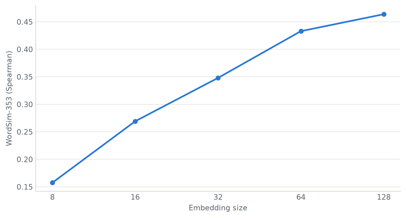
Figure 2: One variable changed, everything else held fixed. Five runs answer the question forty-eight could not.

for a, b in zip(DIMENSIONS, DIMENSIONS[1:]):
    gain = scores[DIMENSIONS.index(b)] - scores[DIMENSIONS.index(a)]
    print(f"{a:>4} -> {b:<4} doubles the size and buys {gain:+.4f}")

   8 -> 16   doubles the size and buys +0.1118
  16 -> 32   doubles the size and buys +0.0789
  32 -> 64   doubles the size and buys +0.0850
  64 -> 128  doubles the size and buys +0.0308

That is a curve, and it says something specific: every doubling helps, and the help is shrinking. The first doubling is worth roughly three times the last, and the fall-off only really arrives past 64 — which is a more useful thing to know than a single recommended number, because it tells you what the next doubling would cost you to find out.

Two caveats worth stating, because the number is easy to over-read.

This corpus is small. A fiftieth of text8, and only 3,704 words survive the minimum-count threshold. A vocabulary that small needs fewer dimensions to separate, so the saturation point here is lower than it would be on the full corpus. The shape transfers; the elbow doesn’t.

WordSim-353 only covers part of this vocabulary. A third of its pairs contain a word this corpus never saw often enough, so the score is computed on the pairs that are left.

What I’d actually take away

A hyperparameter search and an experiment are different things, and they look the same from the outside. Both produce a table of configurations and scores. But a search is trying to be unbalanced — that’s the mechanism by which it finds a good model quickly — and an unbalanced table cannot tell you what an individual knob does. The runs you would need are the ones it correctly declined to spend budget on.

The controlled version is cheap. Five runs against forty-eight. I had assumed answering this properly would be expensive, and the expensive thing was the search that couldn’t answer it.

Ask the search for what it’s good at. The same sweep did tell me something valuable, by accident: window size and negative count barely moved the score between their best and worst settings anywhere in the table. That’s a robustness observation, and a badly balanced search is fine for noticing which knobs are not worth another twelve hours.

The sweep, the trainer and the benchmarks are on GitHub.

Built:      2026-09-18 02:23:27 UTC
Python:     3.13.15
matplotlib: 3.11.2
numpy:      2.5.3
torch:      2.14.0+cpu