An image is not a sequence, so you make it one

Week 3 was a Vision Transformer built from scratch. The whole idea fits in one move at the very start, and you can see it working on a model small enough to train while this page loads.

Week 3: take the transformer, which was designed for text, and point it at images. No convolutions.

The awkward part is that a transformer eats a sequence of tokens, and an image isn’t one. It’s a grid of pixels with no natural order and far too many of them — 28×28 is 784 pixels, and attention costs grow with the square of the sequence length. On a real photograph you’d be computing attention over hundreds of thousands of positions.

The Vision Transformer paper [1] solves this in one move, in the first layer, and everything after it is the ordinary transformer with nothing changed: cut the image into fixed-size squares and treat each square as a word.

import sys

sys.path.insert(0, "..")
import numpy as np
import torch
import torch.nn as nn
from huggingface_hub import hf_hub_download

REVISION = "f705fed08827ff6c36e3b5329495c943a5e544e8"
path = hf_hub_download("roshbeed/ai-residency-blog-data", "mnist/mnist-small.npz",
                       repo_type="dataset", revision=REVISION)
data = np.load(path)

x_train = torch.from_numpy(data["x_train"]).float() / 255.0
y_train = torch.from_numpy(data["y_train"]).long()
x_test = torch.from_numpy(data["x_test"]).float() / 255.0
y_test = torch.from_numpy(data["y_test"]).long()

PATCH = 7
PATCHES = (28 // PATCH) ** 2


def patchify(images):
    """28x28 -> 16 patches of 7x7, flattened. This is the whole trick."""
    batch = images.shape[0]
    tiles = images.unfold(1, PATCH, PATCH).unfold(2, PATCH, PATCH)
    return tiles.reshape(batch, PATCHES, PATCH * PATCH)


baseline = torch.bincount(y_test).max().item() / len(y_test)
print(f"{len(x_train):,} training digits, {len(x_test):,} test digits")
print(f"each image becomes {PATCHES} tokens of {PATCH * PATCH} numbers")
print(f"always guessing the most common digit: {baseline:.4f}")

6,000 training digits, 1,500 test digits
each image becomes 16 tokens of 49 numbers
always guessing the most common digit: 0.1173

import matplotlib.pyplot as plt
from _style import COLOURS, MUTED

digit = x_train[1]
tiles = patchify(digit.unsqueeze(0))[0].reshape(4, 4, PATCH, PATCH)

fig = plt.figure(figsize=(7.2, 3.6))
outer = fig.add_gridspec(1, 2, wspace=0.15)

whole = fig.add_subplot(outer[0])
whole.imshow(digit, cmap="gray_r")
whole.set_title("the image", fontsize=10, color=MUTED, pad=8)
whole.axis("off")

inner = outer[1].subgridspec(4, 4, wspace=0.18, hspace=0.18)
for r in range(4):
    for c in range(4):
        ax = fig.add_subplot(inner[r, c])
        ax.imshow(tiles[r, c], cmap="gray_r", vmin=0, vmax=1)
        ax.set_xticks([]); ax.set_yticks([])
        for s in ax.spines.values():
            s.set_color("#cfd4da")
        if r == 0 and c == 1:
            ax.set_title("sixteen tokens", fontsize=10, color=MUTED, pad=8, loc="left")

Figure 1: One digit as the model sees it: sixteen 7x7 patches, which become sixteen tokens in a sequence.

Each patch gets projected to a vector by a single Linear, and from there the model has a sequence of 16 vectors — structurally identical to a sentence of 16 words. A [CLS] token is stuck on the front, exactly as BERT does, and its final representation is what the classifier reads.

The project version wrote the attention, the encoder block and the positional encodings by hand, with no torch.nn.Transformer anywhere. Here I use the built-in attention, because this post is about the patching idea rather than the arithmetic inside a head.

DIM, HEADS, LAYERS = 64, 4, 2


class Block(nn.Module):
    def __init__(self):
        super().__init__()
        self.attention = nn.MultiheadAttention(DIM, HEADS, batch_first=True)
        self.norm1, self.norm2 = nn.LayerNorm(DIM), nn.LayerNorm(DIM)
        self.feedforward = nn.Sequential(nn.Linear(DIM, 4 * DIM), nn.GELU(),
                                         nn.Linear(4 * DIM, DIM))

    def forward(self, x, want_weights=False):
        attended, weights = self.attention(x, x, x, need_weights=want_weights,
                                           average_attn_weights=True)
        x = self.norm1(x + attended)
        return self.norm2(x + self.feedforward(x)), weights


class VisionTransformer(nn.Module):
    def __init__(self, use_positions=True):
        super().__init__()
        self.use_positions = use_positions
        self.project = nn.Linear(PATCH * PATCH, DIM)
        self.cls = nn.Parameter(torch.zeros(1, 1, DIM))
        self.positions = nn.Parameter(torch.randn(1, PATCHES + 1, DIM) * 0.02)
        self.blocks = nn.ModuleList([Block() for _ in range(LAYERS)])
        self.head = nn.Linear(DIM, 10)

    def forward(self, images, want_weights=False):
        tokens = self.project(patchify(images))
        tokens = torch.cat([self.cls.expand(len(images), -1, -1), tokens], dim=1)
        if self.use_positions:
            tokens = tokens + self.positions

        weights = None
        for i, block in enumerate(self.blocks):
            tokens, w = block(tokens, want_weights and i == LAYERS - 1)
            if w is not None:
                weights = w
        return self.head(tokens[:, 0]), weights  # position 0 is the [CLS] token

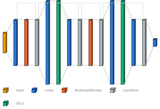
Drawn out, with the shapes the tensors actually take:

from _arch import diagram

diagram(VisionTransformer(), input_shape=(1, 28, 28), style="flow")

Figure 2: The whole model, left to right. Each patch is projected to 64 numbers, two identical encoder blocks run over the 17 tokens, and the head reads position 0. The tall blue-and-green pairs are the feed-forward expansion to 256 inside each block; the outlines spanning the top are the residual connections.

def train(use_positions, epochs=15, batch=128, seed=0):
    torch.manual_seed(seed)
    model = VisionTransformer(use_positions)
    optimiser = torch.optim.AdamW(model.parameters(), lr=3e-3, weight_decay=0.01)
    generator = torch.Generator().manual_seed(seed)

    accuracies = []
    for _ in range(epochs):
        perm = torch.randperm(len(x_train), generator=generator)
        for i in range(0, len(perm) - batch, batch):
            b = perm[i:i + batch]
            loss = nn.functional.cross_entropy(model(x_train[b])[0], y_train[b])
            optimiser.zero_grad()
            loss.backward()
            optimiser.step()
        with torch.no_grad():
            accuracies.append((model(x_test)[0].argmax(1) == y_test).float().mean().item())
    return model, accuracies


model, with_positions = train(use_positions=True)
print(f"{sum(p.numel() for p in model.parameters()):,} parameters")
print(f"best test accuracy: {max(with_positions):.4f}   (baseline {baseline:.4f})")

104,970 parameters
best test accuracy: 0.9393   (baseline 0.1173)

About a hundred thousand parameters, six thousand training images, and a few seconds. The real project got 91.78% on the full MNIST test set after one epoch; this gets to roughly the same place on a fiftieth of the data.

What the position embeddings are for

Self-attention has no idea where anything is. It computes how much each token should attend to each other token, and that calculation is permutation invariant — shuffle the tokens and you get the same set of outputs back, shuffled. Without something to break that symmetry, a Vision Transformer sees a bag of patches, not a picture.

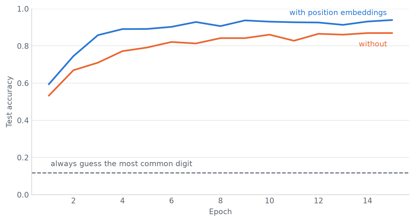
That is what the learned position embeddings do, and you can measure exactly what they are worth by removing them.

_, without_positions = train(use_positions=False)

print(f"with position embeddings:    {max(with_positions):.4f}")
print(f"without position embeddings: {max(without_positions):.4f}")
print(f"difference:                  {max(with_positions) - max(without_positions):+.4f}")

with position embeddings:    0.9393
without position embeddings: 0.8693
difference:                  +0.0700

from _style import figure, style_axes

epochs = range(1, len(with_positions) + 1)
fig, ax = figure(height=3.8)
ax.axhline(baseline, color=MUTED, linewidth=1.2, linestyle="--")
ax.plot(epochs, with_positions, color=COLOURS[0], linewidth=2)
ax.plot(epochs, without_positions, color=COLOURS[1], linewidth=2)
ax.annotate("with position embeddings", xy=(epochs[-1], with_positions[-1]),
            xytext=(-6, 6), textcoords="offset points", ha="right",
            fontsize=9, color=COLOURS[0])
ax.annotate("without", xy=(epochs[-1], without_positions[-1]), xytext=(-6, -16),
            textcoords="offset points", ha="right", fontsize=9, color=COLOURS[1])
ax.annotate("always guess the most common digit", xy=(1, baseline), xytext=(2, 8),
            textcoords="offset points", fontsize=9, color=MUTED)
ax.set_ylim(0, 1.0)
style_axes(ax, "Epoch", "Test accuracy")
fig.tight_layout()

Figure 3: The same model trained with and without position embeddings. Without them the model can still recognise which patches are present, just not where.

It still works without them, which surprised me at first — and then made sense. A bag of 7×7 patches carries a lot about which digit it is, because a 0 and a 1 contain visibly different patches regardless of arrangement. The position embeddings are worth the last several points, which is where the distinctions that depend on layout live.

What the CLS token looks at

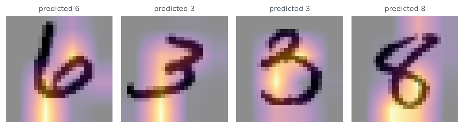
Since the classifier reads only position 0, the attention weights out of that position say which patches the model is actually using.

with torch.no_grad():
    logits, weights = model(x_test[:4], want_weights=True)

cls_attention = weights[:, 0, 1:].reshape(-1, 4, 4)  # row 0 = the [CLS] token

fig, axes = plt.subplots(1, 4, figsize=(8.2, 2.4))
for ax, image, attention, predicted in zip(axes, x_test[:4], cls_attention, logits.argmax(1)):
    ax.imshow(image, cmap="gray_r")
    ax.imshow(attention, cmap="inferno", alpha=0.45, extent=(0, 28, 28, 0),
              interpolation="bilinear")
    ax.set_title(f"predicted {predicted.item()}", fontsize=9, color=MUTED, pad=6)
    ax.axis("off")
fig.tight_layout()

Figure 4: Attention from the [CLS] token in the final block, for four test digits. Brighter patches are the ones the classification actually rests on.

The attention concentrates on the patches with ink in them and largely ignores the empty corners, which is the behaviour you’d want and nobody specified. Nothing in the loss says “look at the strokes” — it falls out of training the classifier.

I’d be careful about reading much more than that into it. Attention maps are suggestive, not explanatory, and with two layers and sixteen patches this one is very coarse.

The part that transfers

The reason this architecture mattered isn’t MNIST accuracy — a small CNN beats it easily at this scale, and the ViT paper is explicit that transformers only overtake convolutional networks with a lot of data behind them.

It’s that once an image is a sequence of tokens, it is the same kind of object as a sentence. That’s what makes it possible to feed images and text to one model, which is where week 4 goes.

The full project, with the attention and encoder blocks written from scratch, is on GitHub.

---

[1] Dosovitskiy et al. An Image is Worth 16x16 Words: Transformers for Image Recognition at Scale. ICLR 2021.

Built:      2026-09-18 02:24:25 UTC
Python:     3.13.15
matplotlib: 3.11.2
numpy:      2.5.3
torch:      2.14.0+cpu