The loss went to zero and the model had learned nothing

Week 2 was a two-tower retrieval system. Building it was straightforward. The part worth writing down is how convincingly the training loss lied about whether it was working.

Week 2: build the thing behind semantic search. Given a query, find the passage in a corpus that answers it.

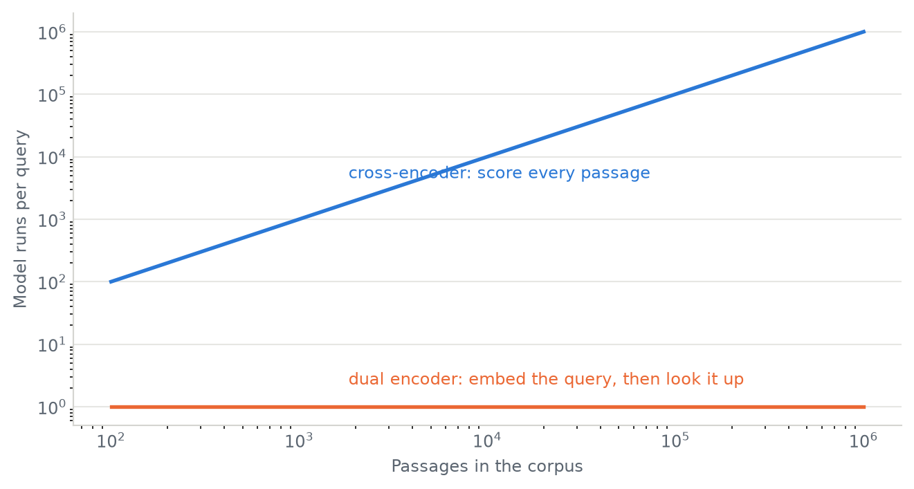
The obvious approach is to take the query and a candidate passage, feed both into one model, and let it score the pair. That works well and is completely impractical, because you have to run it once for every passage in the corpus, for every query.

The dual encoder gets around it by refusing to let the query and the document meet. Two separate towers, one for each, both producing a vector in the same space. A query is relevant to a passage if their vectors are close.

That constraint is the whole point: because the document tower never sees the query, you can run it before any query exists. Embed the entire corpus once, offline, put the vectors in an index, and at query time you embed one short string and do a nearest-neighbour lookup.

import sys

sys.path.insert(0, "..")
import numpy as np
from _style import COLOURS, MUTED, figure, style_axes

corpus = np.logspace(2, 6, 200)

fig, ax = figure(height=3.8)
ax.plot(corpus, corpus, color=COLOURS[0], linewidth=2)
ax.plot(corpus, np.ones_like(corpus), color=COLOURS[1], linewidth=2)
ax.annotate("cross-encoder: score every passage", xy=(2000, 2000), xytext=(-4, 12),
            textcoords="offset points", fontsize=9, color=COLOURS[0])
ax.annotate("dual encoder: embed the query, then look it up", xy=(2000, 1),
            xytext=(-4, 12), textcoords="offset points", fontsize=9, color=COLOURS[1])
ax.set_xscale("log")
ax.set_yscale("log")
style_axes(ax, "Passages in the corpus", "Model runs per query")
fig.tight_layout()

Figure 1: Model runs needed to answer one query. The cross-encoder has to score every passage; the dual encoder embeds the query once and lets an index do the rest.

Training it: triplet loss

The towers start out random, so you have to teach them what close means. The signal used in the project is a triplet: a query, a passage that answers it, and a passage that doesn’t. Push the first pair together and the second apart, by at least a margin \(m\):

\[\mathcal{L} = \max\big(0,\ m - s(q, d^{+}) + s(q, d^{-})\big)\]

If the positive is already more similar than the negative by the margin, the loss is zero and nothing happens. Otherwise both towers get nudged.

A toy corpus with free labels

Real retrieval training needs query-passage pairs, which is the expensive part. There’s a standard trick for getting them free: take a document, cut a piece out, and use the piece as the query. It’s called the inverse cloze task [1], and it’s how several retrieval models get pre-trained.

Here I take Hacker News titles of at least eight words and cut them in half. The first half is the query, the second half is the document it should retrieve. No labelling, and the two halves are genuinely about the same thing.

import gzip
import json
import re
import zlib

import torch
import torch.nn as nn
import torch.nn.functional as F
from huggingface_hub import hf_hub_download

REVISION = "f705fed08827ff6c36e3b5329495c943a5e544e8"
path = hf_hub_download("roshbeed/ai-residency-blog-data", "hn/hn-sample.json.gz",
                       repo_type="dataset", revision=REVISION)
rows = json.load(gzip.open(path, "rt"))
titles = [r["title"] for r in rows["train"]] + [r["title"] for r in rows["test"]]

tokenise = lambda s: re.findall(r"[a-z0-9\+#]+", s.lower())
pairs = []
for title in titles:
    words = tokenise(title)
    if len(words) >= 8:
        half = len(words) // 2
        pairs.append((words[:half], words[half:]))

print(f"{len(pairs):,} query/document pairs")
print(f"  query:    {' '.join(pairs[0][0])}")
print(f"  document: {' '.join(pairs[0][1])}")

79,009 query/document pairs
  query:    california governor to deploy 500 surveillance
  document: cameras to oakland to fight crime

DIM = 2**14


def encode(sequences):
    """Bag of hashed words. crc32 rather than hash() — Python's is salted per process."""
    X = torch.zeros(len(sequences), DIM)
    for i, words in enumerate(sequences):
        for w in words:
            X[i, zlib.crc32(w.encode()) % DIM] += 1.0
        if words:
            X[i] /= len(words)
    return X


rng = np.random.default_rng(0)
order = rng.permutation(len(pairs))
train_ids, test_ids = order[:40_000], order[40_000:45_000]

Q = encode([pairs[i][0] for i in train_ids])
D = encode([pairs[i][1] for i in train_ids])
Q_test = encode([pairs[i][0] for i in test_ids])
D_test = encode([pairs[i][1] for i in test_ids])

print(f"{len(Q):,} training pairs, {len(D_test):,} documents to search at test time")

40,000 training pairs, 5,000 documents to search at test time

class Tower(nn.Module):
    """Text in, a unit vector out. Query and document get one of these each."""

    def __init__(self, out=128):
        super().__init__()
        self.net = nn.Sequential(nn.Linear(DIM, 256), nn.ReLU(), nn.Linear(256, out))

    def forward(self, x):
        return F.normalize(self.net(x), dim=-1)


def recall_at_10(query_tower, doc_tower):
    """How often the right document is in the top 10 of all 5,000."""
    with torch.no_grad():
        similarity = query_tower(Q_test) @ doc_tower(D_test).T
        top = similarity.topk(10, dim=1).indices
        correct = torch.arange(len(Q_test)).unsqueeze(1)
        return (top == correct).any(1).float().mean().item()


CHANCE = 10 / len(D_test)
print(f"chance recall@10 = {CHANCE:.4f}")

chance recall@10 = 0.0020

from _arch import diagram

diagram(Tower(), input_shape=(1, DIM))

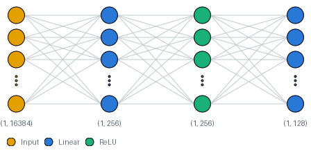
Figure 2: One tower. Both the query and the document side are this same shape, with separate weights, and the output is normalised to unit length so a dot product is a cosine.

def train(loss_fn, epochs=8, batch=256, seed=0):
    torch.manual_seed(seed)
    query_tower, doc_tower = Tower(), Tower()
    optimiser = torch.optim.Adam([*query_tower.parameters(), *doc_tower.parameters()], lr=1e-3)
    generator = torch.Generator().manual_seed(seed)

    losses, recalls = [], []
    for _ in range(epochs):
        perm = torch.randperm(len(Q), generator=generator)
        total = steps = 0
        for i in range(0, len(perm) - batch, batch):
            b = perm[i:i + batch]
            loss = loss_fn(query_tower, doc_tower, b, perm, generator)
            optimiser.zero_grad()
            loss.backward()
            optimiser.step()
            total += loss.item()
            steps += 1
        losses.append(total / steps)
        recalls.append(recall_at_10(query_tower, doc_tower))
    return losses, recalls


MARGIN = 0.2


def triplet(query_tower, doc_tower, b, perm, generator):
    """The project's loss: one random passage as the negative."""
    negatives = perm[torch.randperm(len(b), generator=generator)]
    q = query_tower(Q[b])
    positive = (q * doc_tower(D[b])).sum(-1)
    negative = (q * doc_tower(D[negatives])).sum(-1)
    return F.relu(MARGIN - positive + negative).mean()


triplet_loss, triplet_recall = train(triplet)
for epoch, (l, r) in enumerate(zip(triplet_loss, triplet_recall), 1):
    print(f"epoch {epoch}: loss {l:.4f}   recall@10 {r:.4f}   ({r / CHANCE:.1f}x chance)")

epoch 1: loss 0.0121   recall@10 0.0020   (1.0x chance)
epoch 2: loss 0.0093   recall@10 0.0022   (1.1x chance)
epoch 3: loss 0.0123   recall@10 0.0022   (1.1x chance)
epoch 4: loss 0.0199   recall@10 0.0020   (1.0x chance)
epoch 5: loss 0.0142   recall@10 0.0020   (1.0x chance)
epoch 6: loss 0.0201   recall@10 0.0018   (0.9x chance)
epoch 7: loss 0.0179   recall@10 0.0020   (1.0x chance)
epoch 8: loss 0.0178   recall@10 0.0018   (0.9x chance)

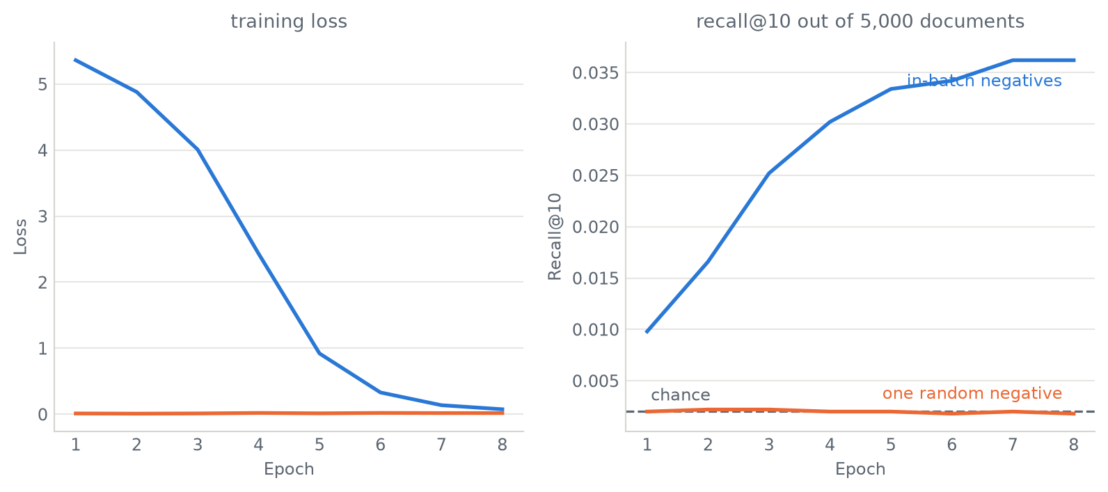
The loss falls to near zero within one epoch, and recall never leaves chance. Out of 5,000 documents, the model finds the right one in its top ten about as often as picking ten at random would.

If you were watching the loss curve — which is the thing that’s easy to watch — you would conclude this was training beautifully.

Why it happens

A negative drawn at random from the corpus is about a different subject entirely. The towers only have to tell “machine learning” from “sourdough starter”, and they can do that almost immediately. Once the margin is satisfied, the loss is exactly zero, and a loss of zero has no gradient.

So the model stops learning while still being unable to do the thing you want, which is to tell the right passage from a thousand plausible ones.

The usual fix is to stop picking one negative and use the whole batch: every other document in the batch is a negative for this query, and the loss becomes a cross-entropy over which of them is correct. It’s a harder question, it stays hard as the model improves, and it costs nothing extra because those documents are already encoded.

TEMPERATURE = 0.05


def in_batch(query_tower, doc_tower, b, perm, generator):
    """Every other document in the batch is a negative for this query."""
    q, docs = query_tower(Q[b]), doc_tower(D[b])
    logits = (q @ docs.T) / TEMPERATURE
    return F.cross_entropy(logits, torch.arange(len(b)))


batch_loss, batch_recall = train(in_batch)
for epoch, (l, r) in enumerate(zip(batch_loss, batch_recall), 1):
    print(f"epoch {epoch}: loss {l:.4f}   recall@10 {r:.4f}   ({r / CHANCE:.1f}x chance)")

epoch 1: loss 5.3608   recall@10 0.0098   (4.9x chance)
epoch 2: loss 4.8804   recall@10 0.0166   (8.3x chance)
epoch 3: loss 4.0087   recall@10 0.0252   (12.6x chance)
epoch 4: loss 2.4321   recall@10 0.0302   (15.1x chance)
epoch 5: loss 0.9204   recall@10 0.0334   (16.7x chance)
epoch 6: loss 0.3301   recall@10 0.0342   (17.1x chance)
epoch 7: loss 0.1374   recall@10 0.0362   (18.1x chance)
epoch 8: loss 0.0757   recall@10 0.0362   (18.1x chance)

import matplotlib.pyplot as plt

epochs = range(1, len(batch_loss) + 1)
fig, (left, right) = plt.subplots(1, 2, figsize=(8.4, 3.8))

left.plot(epochs, triplet_loss, color=COLOURS[1], linewidth=2)
left.plot(epochs, batch_loss, color=COLOURS[0], linewidth=2)
left.set_title("training loss", fontsize=10, color=MUTED, pad=8)
style_axes(left, "Epoch", "Loss")

right.axhline(CHANCE, color=MUTED, linewidth=1.2, linestyle="--")
right.plot(epochs, triplet_recall, color=COLOURS[1], linewidth=2)
right.plot(epochs, batch_recall, color=COLOURS[0], linewidth=2)
right.annotate("in-batch negatives", xy=(epochs[-1], batch_recall[-1]), xytext=(-6, -14),
               textcoords="offset points", ha="right", fontsize=9, color=COLOURS[0])
right.annotate("one random negative", xy=(epochs[-1], triplet_recall[-1]), xytext=(-6, 8),
               textcoords="offset points", ha="right", fontsize=9, color=COLOURS[1])
right.annotate("chance", xy=(1, CHANCE), xytext=(2, 6), textcoords="offset points",
               fontsize=9, color=MUTED)
right.set_title("recall@10 out of 5,000 documents", fontsize=10, color=MUTED, pad=8)
style_axes(right, "Epoch", "Recall@10")

fig.tight_layout()

Figure 3: The same towers, the same data, the same number of steps. Only the choice of negatives differs.

Same towers, same data, same number of gradient steps. The only change is which documents count as negatives, and it’s the difference between a model that works and a model that doesn’t.

Note what the loss curves do. The triplet loss ends lower than the in-batch loss. If you ranked these two runs by final training loss you would pick the one that learned nothing.

Why this matters beyond the toy

Negative sampling is the part of contrastive training that looks like a detail and isn’t. The architecture — two towers, a shared space, an index — is the easy half and mostly writes itself. What decides whether the thing retrieves anything is the question you ask it during training, and “is this passage more relevant than one picked at random” is not a hard enough question to learn from.

That’s why the literature moved to in-batch negatives and then to actively mined hard negatives: passages that look plausible for the query and aren’t. Each step makes the training question harder in the same direction.

The general lesson I took from this one, and now apply everywhere: report a metric next to the number a model that learned nothing would get. Chance recall@10 over 5,000 documents is 0.002. Any recall figure without that 0.002 beside it is unreadable — and a falling loss beside it is worth nothing at all.

The full project, with the GRU towers, the sweep and the Redis index, is on GitHub.

---

[1] Lee, Chang, Toutanova. Latent Retrieval for Weakly Supervised Open Domain Question Answering. ACL 2019.

Built:      2026-09-18 02:28:47 UTC
Python:     3.13.15
matplotlib: 3.11.2
numpy:      2.5.3
torch:      2.14.0+cpu