A good title doesn’t add upvotes, it multiplies them

The second half of week 1 was predicting Hacker News scores from a post’s title and its metadata. The interesting part turned out to be a question about architecture: where in the model should the two kinds of input meet?

The second project of week 1: given a Hacker News post — its title, where it links, when it was submitted and who by — predict how many upvotes it will get.

872,554 real posts, split by time so the model is always predicting a future it hasn’t seen. The served model’s median error is 10.1 upvotes against 16.2 for guessing the average every time.

But the number isn’t what made this project interesting. The interesting part was a design question I didn’t expect to have to think about: a post is two different kinds of thing at once — a piece of text, and a handful of numbers and categories. Where in the model should they meet?

Early and late fusion

The multimodal literature has names for the two ends of this. In Snoek et al.’s 2005 survey of video retrieval [1], which is where the terms come from:

Early fusion glues the inputs together first and runs one model over the whole thing. The model can learn anything that depends on both — but it also has to learn the text and the metadata in the same layers, entangled from the start.

Late fusion gives each input its own model, reduces each to a score, and combines the scores at the end. Clean, modular, and you can retrain one branch without touching the other.

Snoek’s objection to late fusion is the one that matters: by the time the two branches meet, each has been squeezed into a single number, so any correlation between the two in feature space is already gone.

They’re the same architecture with a switch

The thing that made this tractable for me was realising early and late fusion aren’t two designs. Late fusion is early fusion with some weights deleted.

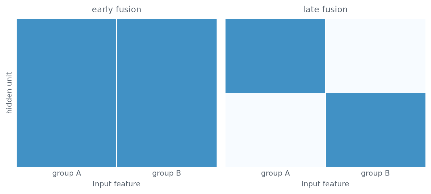
Take one hidden layer over all the inputs concatenated. Early fusion lets every hidden unit see every input. Late fusion splits the units into groups and lets each group see only its own inputs — which is the same layer with the off-diagonal blocks zeroed.

Same inputs, same width, same depth, same head. The only difference is which weights are allowed to be non-zero.

import sys

sys.path.insert(0, "..")
import matplotlib.pyplot as plt
import numpy as np
import torch
from _style import COLOURS, MUTED

D, H = 6, 64


def mask_for(kind):
    """Which first-layer weights are allowed to be non-zero."""
    mask = torch.ones(2 * D, H)
    if kind == "late":
        mask[:D, H // 2:] = 0   # the first half of the units sees group A only
        mask[D:, :H // 2] = 0   # the second half sees group B only
    return mask


fig, axes = plt.subplots(1, 2, figsize=(7.4, 3.4))
for ax, kind, title in zip(axes, ("early", "late"), ("early fusion", "late fusion")):
    ax.imshow(mask_for(kind).T, aspect="auto", cmap="Blues", vmin=0, vmax=1.6)
    ax.set_title(title, fontsize=10, color=MUTED, pad=8)
    ax.set_xlabel("input feature", color=MUTED, fontsize=9)
    ax.axvline(D - 0.5, color="white", linewidth=1.5)
    ax.set_xticks([D / 2 - 0.5, D * 1.5 - 0.5]); ax.set_xticklabels(["group A", "group B"])
    ax.set_yticks([])
    ax.tick_params(colors=MUTED, labelsize=9, length=0)
    for s in ax.spines.values():
        s.set_visible(False)
axes[0].set_ylabel("hidden unit", color=MUTED, fontsize=9)
fig.tight_layout()

Figure 1: The first weight matrix of each architecture. Late fusion is the same matrix with the cross-group blocks held at zero.

Written this way the question stops being “which architecture” and becomes “does this task need those cross-group weights?” — which is something you can measure.

A task where the answer is known

Before measuring anything on real data, it’s worth checking the measurement works on a target where you already know the answer.

So: two groups of random inputs, A and B. Each has a hidden linear score, and the target is

\[y = s_A + s_B + \alpha \cdot s_A s_B\]

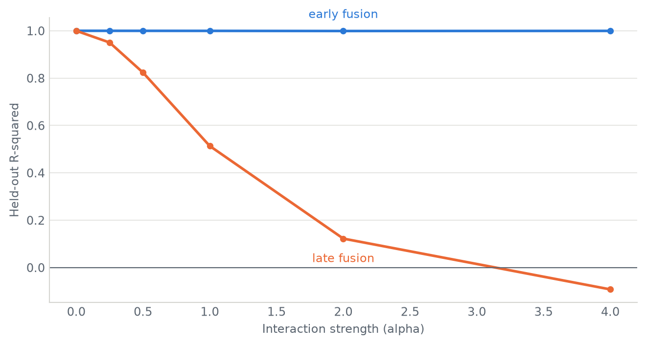
At \(\alpha = 0\) the target is purely additive — the two groups contribute independently, and a model that scores them separately and adds is exactly right. As \(\alpha\) grows, the product term takes over, and a model that can only add should fall further and further behind.

import torch.nn as nn

N = 6000


def make_data(alpha, seed):
    g = torch.Generator().manual_seed(seed)
    a = torch.randn(N, D, generator=g)
    b = torch.randn(N, D, generator=g)
    wa = torch.randn(D, generator=g) / D**0.5
    wb = torch.randn(D, generator=g) / D**0.5

    score_a, score_b = a @ wa, b @ wb
    y = score_a + score_b + alpha * score_a * score_b
    return torch.cat([a, b], 1), (y - y.mean()) / y.std()


class Fusion(nn.Module):
    """One architecture. `kind` only decides which weights may be non-zero."""

    def __init__(self, kind, seed):
        super().__init__()
        torch.manual_seed(seed)
        self.first = nn.Linear(2 * D, H)
        self.head = nn.Linear(H, 1)
        self.register_buffer("mask", mask_for(kind))

    def forward(self, x):
        hidden = torch.relu(x @ (self.first.weight.T * self.mask) + self.first.bias)
        return self.head(hidden).squeeze(-1)

def variance_explained(kind, alpha, seed, steps=1500):
    X, y = make_data(alpha, seed)
    split = int(0.7 * N)
    model = Fusion(kind, 100 + seed)
    optimiser = torch.optim.Adam(model.parameters(), lr=0.02)

    for _ in range(steps):
        loss = ((model(X[:split]) - y[:split]) ** 2).mean()
        optimiser.zero_grad()
        loss.backward()
        optimiser.step()

    with torch.no_grad():  # R² on the held-out third
        return 1 - ((model(X[split:]) - y[split:]) ** 2).mean().item() / y[split:].var().item()


alphas = [0.0, 0.25, 0.5, 1.0, 2.0, 4.0]
early = [np.median([variance_explained("early", a, s) for s in range(3)]) for a in alphas]
late = [np.median([variance_explained("late", a, s) for s in range(3)]) for a in alphas]

print(f"{'alpha':>6} {'early':>8} {'late':>8} {'gap':>8}")
for a, e, l in zip(alphas, early, late):
    print(f"{a:>6} {e:>8.4f} {l:>8.4f} {e - l:>+8.4f}")

 alpha    early     late      gap
   0.0   1.0000   1.0000  -0.0000
  0.25   0.9999   0.9504  +0.0495
   0.5   0.9998   0.8302  +0.1697
   1.0   0.9997   0.5019  +0.4978
   2.0   0.9995   0.1125  +0.8870
   4.0   0.9995  -0.0717  +1.0711

from _style import figure, style_axes

fig, ax = figure(height=3.8)
ax.plot(alphas, early, color=COLOURS[0], linewidth=2, marker="o", markersize=4)
ax.plot(alphas, late, color=COLOURS[1], linewidth=2, marker="o", markersize=4)
ax.annotate("early fusion", xy=(alphas[-2], early[-2]), xytext=(0, 10),
            textcoords="offset points", fontsize=9, color=COLOURS[0], ha="center")
ax.annotate("late fusion", xy=(alphas[-2], late[-2]), xytext=(0, -18),
            textcoords="offset points", fontsize=9, color=COLOURS[1], ha="center")
ax.axhline(0, color=MUTED, linewidth=0.8)
style_axes(ax, "Interaction strength (alpha)", "Held-out R-squared")
fig.tight_layout()

Figure 2: Held-out R² as the interaction term grows. With no interaction the two are identical; the gap is entirely the product term.

At \(\alpha = 0\) the two are indistinguishable — both fit the additive target essentially perfectly. Deleting the cross-group weights costs nothing when there is nothing across the groups to model.

Everything after that is the interaction, and it is not subtle: by \(\alpha = 4\) late fusion is explaining none of the held-out variance at all. It isn’t that it fits the product term badly. It cannot represent it, at any width.

So does Hacker News have one?

That was the real question, and the answer is yes, in one specific place: the title and the timing. Fitting the same comparison on the real upvote counts, for every pairing of input groups, the title-times-timing cell was the largest effect in the table — +0.038 Spearman for a model that can represent the interaction over one that can’t.

The mechanism makes sense once you look at the distribution. The same title is worth a handful of points at a dead hour and hundreds when the site is awake. A good title doesn’t add a fixed number of upvotes — it multiplies whatever the timing was going to give you. A model that scores the title and the metadata separately and sums the two scores can only add, so it splits the difference and is wrong in both directions.

There’s a catch that took me a while to get straight, and it’s the most useful thing I learned on this project.

Additivity is a property of your units, not of your data. Fit the exact same comparison on log1p(score) instead of the raw count and every interaction disappears — because a logarithm turns multiplication into addition. Fit it on rank and they vanish too, since rank keeps every comparison and throws away all the magnitudes.

So the interaction lives in how big the numbers get, not in which post beats which. If this service ranked posts, it would not need early fusion. It predicts counts, so it does.

What the toy above can’t show you

I tried to reproduce the real finding at the scale of this page — 100,000 posts, a hashed bag of words for the title, hour and weekday for the timing — and it isn’t there. The joint model comes out slightly behind the additive one.

That’s not a contradiction, it’s a lesson about effect sizes. +0.038 Spearman is small next to the seed-to-seed spread of these models, which is why the real measurement needed ten seeds per cell and a capacity-matched control, and why the whole question took a few thousand runs to answer rather than a few dozen.

The synthetic target above is the honest version of what a toy can do here: it shows you the mechanism clearly, on data built so the mechanism is the only thing present. It can’t tell you how much of that mechanism is in a real dataset.

The ceiling

The other thing worth knowing about this task: Hacker News is substantially a lottery. The same link posted twice scores similarly only about a quarter of the time. Whatever the architecture, there’s a hard bound on what any model can do here, and it’s a lot lower than you’d hope.

The full project — the fusion sweep, the four baselines, the deployed API — is on GitHub.

---

[1] Snoek, Worring, Smeulders. Early versus Late Fusion in Semantic Video Analysis. ACM Multimedia 2005.

Built:      2026-09-18 01:36:12 UTC
Python:     3.13.15
matplotlib: 3.11.2
numpy:      2.5.3
torch:      2.14.0+cpu