What the KL penalty is actually holding back

Week 6 was PPO for RLHF, built one module at a time. The clipped objective gets the attention, but the term that decides whether you get a useful model or a slot machine is the other one.

Week 6, the last one: reinforcement learning from human feedback. The loop that turned GPT-3 into InstructGPT [1], built from scratch — generation, KL penalty, reward, advantage estimation, and the clipped policy and value updates, one small module each.

The reason RL shows up here at all is that you can’t write down a loss for “a good summary”. What you can do is show people two summaries and ask which they prefer, train a model to predict those preferences, and then optimise the language model against that.

Which introduces the problem the whole method is organised around: you are now optimising a learned approximation of what you want. Push hard enough on any learned reward and you stop finding good outputs and start finding its mistakes.

A language, and a reward model with a weakness

To watch that happen I need something that has grammar, and a reward model that is slightly wrong about what’s good.

The language: eight tokens, where each one usually follows the one before it — token 4 tends to be followed by 5, then 6, and so on. A small bigram model trained on samples of it is the reference policy, standing in for the supervised model you start RLHF from.

The reward model: it likes token 3. That’s it. Think of it as a preference model that has correctly noticed people enjoy a particular thing, and has no opinion about anything else — which is roughly how real reward models fail.

import sys

sys.path.insert(0, "..")
import numpy as np
import torch
import torch.nn as nn
import torch.nn.functional as F

VOCAB, LENGTH, START = 8, 6, 0

rng = np.random.default_rng(0)
grammar = np.full((VOCAB, VOCAB), 0.02)
for i in range(VOCAB):
    grammar[i, (i + 1) % VOCAB] = 0.70     # the usual next token
    grammar[i, (i + 2) % VOCAB] = 0.16     # sometimes it skips one
grammar /= grammar.sum(1, keepdims=True)


def sample_corpus(n):
    out = np.zeros((n, LENGTH), int)
    for i in range(n):
        previous = START
        for t in range(LENGTH):
            previous = rng.choice(VOCAB, p=grammar[previous])
            out[i, t] = previous
    return torch.from_numpy(out)


class Bigram(nn.Module):
    def __init__(self):
        super().__init__()
        self.logits = nn.Parameter(torch.zeros(VOCAB, VOCAB))

    def forward(self, previous):
        return self.logits[previous]


corpus = sample_corpus(4000)
torch.manual_seed(0)
reference = Bigram()
optimiser = torch.optim.Adam(reference.parameters(), lr=0.1)
shifted = torch.cat([torch.full((len(corpus), 1), START), corpus[:, :-1]], dim=1)

for _ in range(400):
    loss = F.cross_entropy(reference(shifted).reshape(-1, VOCAB), corpus.reshape(-1))
    optimiser.zero_grad()
    loss.backward()
    optimiser.step()

for p in reference.parameters():
    p.requires_grad_(False)

REWARDED = 3
print(f"reference model trained, cross-entropy {loss.item():.4f}")
print(f"the reward model gives one point per token {REWARDED}, so the maximum is {LENGTH}")

reference model trained, cross-entropy 1.0112
the reward model gives one point per token 3, so the maximum is 6

def reward(sequences):
    return (sequences == REWARDED).float().sum(1)


@torch.no_grad()
def generate(model, n, generator):
    sequences = torch.zeros(n, LENGTH, dtype=torch.long)
    log_probs = torch.zeros(n, LENGTH)
    previous = torch.full((n,), START)
    for t in range(LENGTH):
        lp = F.log_softmax(model(previous), -1)
        nxt = torch.multinomial(lp.exp(), 1, generator=generator).squeeze(1)
        sequences[:, t] = nxt
        log_probs[:, t] = lp.gather(1, nxt[:, None]).squeeze(1)
        previous = nxt
    return sequences, log_probs


def log_prob_of(model, sequences):
    previous = torch.cat([torch.full((len(sequences), 1), START), sequences[:, :-1]], dim=1)
    lp = F.log_softmax(model(previous), -1)
    return lp.gather(2, sequences[..., None]).squeeze(-1)


@torch.no_grad()
def fluency(sequences):
    """How likely these sequences are under the language the model started from."""
    return log_prob_of(reference, sequences).sum(1).mean().item()


generator = torch.Generator().manual_seed(9)
samples, _ = generate(reference, 512, generator)
print(f"reference: reward {reward(samples).mean():.2f}, fluency {fluency(samples):.2f}")
print(f"  it says things like {samples[0].tolist()} and {samples[1].tolist()}")

reference: reward 0.84, fluency -6.19
  it says things like [4, 0, 1, 2, 6, 7] and [7, 0, 1, 2, 4, 5]

The update

PPO’s headline is the clipped objective. Sample some sequences from the current policy, work out how much better than average each one turned out, and then push their probability up — but only so far.

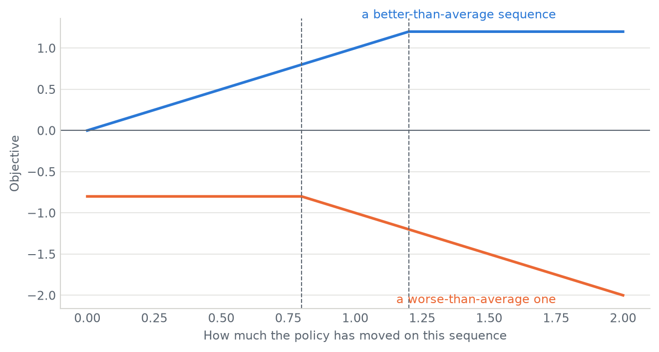
The ratio \(r = \pi_{\text{new}} / \pi_{\text{old}}\) says how much the policy has moved on a sequence since it was sampled. Taking the minimum of \(rA\) and a clipped \(rA\) means that once the policy has moved far enough in the direction the advantage points, there’s no further gradient from that sample. You get to reuse a batch for several steps without the policy running away from the data it was collected from.

from _style import COLOURS, MUTED, figure, style_axes

ratio = np.linspace(0, 2, 400)
CLIP = 0.2

fig, ax = figure(height=3.8)
for advantage, colour, label in ((1.0, COLOURS[0], "a better-than-average sequence"),
                                 (-1.0, COLOURS[1], "a worse-than-average one")):
    objective = np.minimum(ratio * advantage, np.clip(ratio, 1 - CLIP, 1 + CLIP) * advantage)
    ax.plot(ratio, objective, color=colour, linewidth=2)
    ax.annotate(label, xy=(1.75, objective[-40]), xytext=(0, 10 if advantage > 0 else -18),
                textcoords="offset points", ha="right", fontsize=9, color=colour)

for edge in (1 - CLIP, 1 + CLIP):
    ax.axvline(edge, color=MUTED, linewidth=0.8, linestyle="--")
ax.axhline(0, color=MUTED, linewidth=0.8)
style_axes(ax, "How much the policy has moved on this sequence", "Objective")
fig.tight_layout()

Figure 1: The clipped objective, as a function of how far the policy has moved. Once it has moved far enough in the useful direction, the line goes flat and there is nothing more to gain from that sample.

Clipping keeps each update small. It says nothing at all about where the policy ends up after a hundred of them, and that’s the gap the next part lives in.

def train(kl_coefficient, clip=0.2, iterations=120, batch=512, lr=0.05):
    torch.manual_seed(1)
    policy = Bigram()
    policy.logits.data = reference.logits.data.clone()   # start from the reference
    optimiser = torch.optim.Adam(policy.parameters(), lr=lr)
    generator = torch.Generator().manual_seed(2)

    for _ in range(iterations):
        sequences, old_log_prob = generate(policy, batch, generator)
        scores = reward(sequences)
        with torch.no_grad():
            reference_log_prob = log_prob_of(reference, sequences)

        advantage = scores - scores.mean()
        advantage = advantage / (advantage.std() + 1e-8)

        for _ in range(4):        # reuse the batch, which is what clipping makes safe
            new_log_prob = log_prob_of(policy, sequences)
            ratio = (new_log_prob - old_log_prob).exp().sum(1)
            kl = (new_log_prob - reference_log_prob).sum(1)

            clipped = torch.min(ratio * advantage,
                                ratio.clamp(1 - clip, 1 + clip) * advantage)
            loss = -(clipped - kl_coefficient * kl).mean()

            optimiser.zero_grad()
            loss.backward()
            optimiser.step()
    return policy


print(f"{'KL coefficient':>16} {'reward':>8} {'fluency':>9}   a sample")
for coefficient in (0.0, 1.0, 3.0, 6.0, 20.0):
    policy = train(coefficient)
    generator = torch.Generator().manual_seed(9)
    samples, _ = generate(policy, 512, generator)
    label = "none" if coefficient == 0 else f"{coefficient:g}"
    print(f"{label:>16} {reward(samples).mean():>8.2f} {fluency(samples):>9.2f}   "
          f"{samples[0].tolist()}")

generator = torch.Generator().manual_seed(9)
samples, _ = generate(reference, 512, generator)
print(f"{'(reference)':>16} {reward(samples).mean():>8.2f} {fluency(samples):>9.2f}   "
      f"{samples[0].tolist()}")

  KL coefficient   reward   fluency   a sample
            none     6.00    -23.08   [3, 3, 3, 3, 3, 3]
               1     6.00    -23.08   [3, 3, 3, 3, 3, 3]
               3     3.00    -13.73   [1, 3, 1, 3, 1, 3]
               6     2.00     -7.12   [1, 3, 4, 2, 3, 4]
              20     2.00     -5.75   [1, 2, 3, 1, 2, 3]
     (reference)     0.84     -6.19   [4, 0, 1, 2, 6, 7]

Read the samples, not the reward

With no KL penalty the policy scores a perfect 6 out of 6. It does this by saying 3 3 3 3 3 3.

That is the best possible output according to the reward model, and it is not a sentence. Fluency under the original language collapses from −7.5 to −23. The policy has found the reward model’s blind spot and moved in.

Nothing in the reward number tells you this happened. Reward went up monotonically the whole way. If you were watching the metric the run looks like a complete success, and this is why RLHF papers report a KL-to-reference axis next to reward rather than reward alone.

Turn the penalty up and something more interesting than a compromise appears. The policy settles on 2 3 2 3 2 3 — half the maximum reward, and most of the fluency back.

Look at why that particular sequence. In this language, 2 is usually followed by 3. So the policy found a way to say the rewarded token as often as the grammar allows, rather than as often as arithmetic allows. It’s obeying the language and pursuing the reward at the same time.

That’s the whole objective of RLHF in one sequence: not maximum reward, and not the original model, but the best the reward can be served without leaving the distribution the language lives in.

Two things I’d tell myself at the start

Clipping and the KL penalty solve different problems and people conflate them. Clipping bounds how far one update moves the policy from the policy that collected the batch. The KL penalty bounds how far training moves the policy from the model you started with. You can clip perfectly and still walk all the way to 3 3 3 3 3 3, one small safe step at a time — which is exactly what the top row of that table is.

The ratio must score token ids, never re-tokenized text. This one cost me real time. It is natural to record a generated state as its decoded string and re-encode it when computing the ratio, and it looks equivalent. It isn’t: about one in twenty states doesn’t survive decode-then-encode, sometimes coming back with a different number of tokens. The two sides of the ratio were scoring different sequences, so the ratio wasn’t 1 before any gradient step had been taken — and PPO’s entire safety argument rests on it being 1 there.

The full project, with the real reward model and LoRA, is on GitHub.

---

[1] Ouyang et al. Training language models to follow instructions with human feedback. NeurIPS 2022. The PPO algorithm itself is Schulman et al., Proximal Policy Optimization Algorithms, 2017.

Built:      2026-09-18 02:28:55 UTC
Python:     3.13.15
matplotlib: 3.11.2
numpy:      2.5.3
torch:      2.14.0+cpu