The History of Search: From TF-IDF to PageRank to Two-Tower Models

Two towers over query and document, and what changes when every other document in the batch becomes a negative instead of one drawn at random.

The task is to find, given a query, the document that answers it.

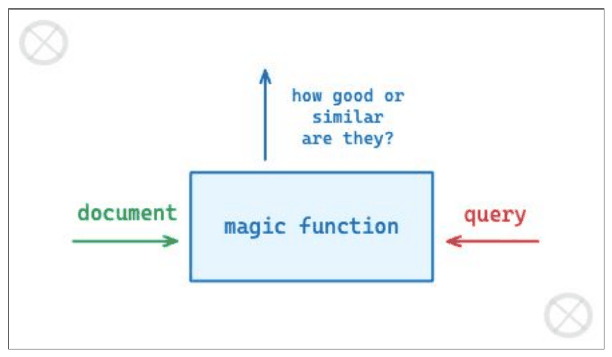
Strip away the machinery and every search system is one function. A document goes in, a query goes in, a number comes out.

Everything in this week is a different way of filling that box in. Rank five documents by running the function five times and sorting.

TF-IDF

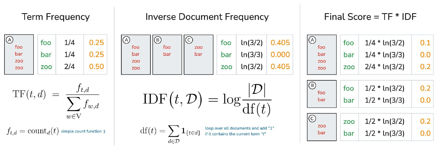
TF-IDF fills the box with counting. Term frequency is how often a query word appears in a document. Inverse document frequency discounts words that appear everywhere: if a term shows up in every document it cannot distinguish between them, so its weight goes to zero. Multiply the two and you have a score, with no learning anywhere.

It also builds an index the other way round, from term to the documents containing it, so answering a query is a lookup rather than a scan of the corpus. That is how search engines worked for decades, and partly still do.

Is It Good Enough?

No, and the reason is in the paper that founded Google:

On the web, this strategy often returns very short documents that are the query plus a few words. For example, we have seen a major search engine return a page containing only “Bill Clinton Sucks” and picture from a “Bill Clinton” query. Some argue that on the web, users should specify more accurately what they want and add more words to their query. We disagree vehemently with this position.

— Brin and Page, The Anatomy of a Large-Scale Hypertextual Web Search Engine, 1998

Counting terms rewards a page for containing the query words. It cannot tell a good page from a bad one that uses the same vocabulary.

The fix is to score the document on its own, separately from the query, using how the rest of the web treats it.

PageRank

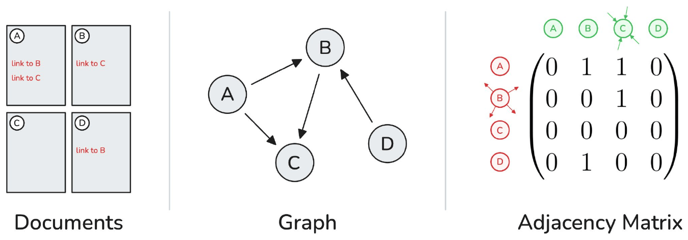
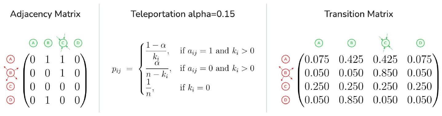
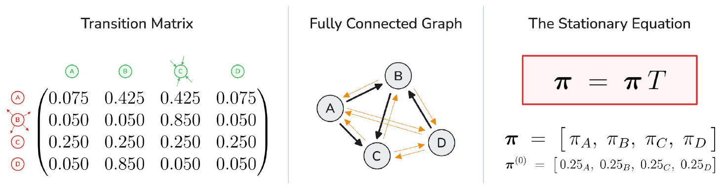
Documents linking to each other form a graph, and a graph is an adjacency matrix. Normalise the rows and that matrix becomes a set of transition probabilities: if you are on page A, where do you go next?

That is a random walk. The teleportation term, \(\alpha = 0.15\), is the chance the walker ignores the links and jumps to a random page instead. Without it the walk can get stuck in a corner of the graph with no way out.

Run the walk forever and the fraction of time spent on each page settles down. That settled distribution is the answer to \(\pi = \pi T\), and it is PageRank: a page is important if a random surfer spends a lot of time there.

The part I found genuinely clarifying is that none of this was new mathematics. Markov described these walks in 1906. PageRank is a standard stationary distribution applied to the link graph, and the teleportation term is there to guarantee the walk has one.

The Other Half

PageRank scores a document on its own merit. It says nothing about whether the document answers this query, and that is still TF-IDF’s job, still by counting words.

So: can we do better than TF-IDF?

The problem with counting is that a query for was ronald reagan a democrat will not match a passage that answers the question without using those exact words. Matching on literal overlap misses meaning.

word2vec had the same problem, and built the answer to it.

CBOW Is an Encoder

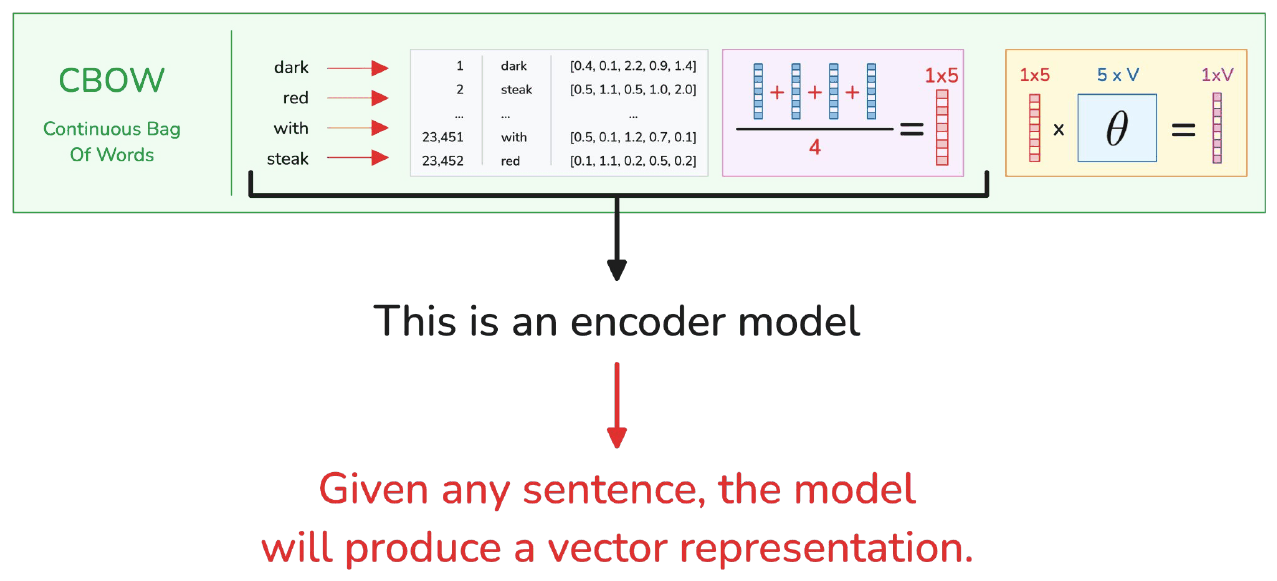
This is the diagram it all turns on.

The CBOW model was built to predict a missing word. But look at what it does on the way: it takes a sentence, looks up a vector per word, and averages them into one vector. That intermediate step was a means to an end, and it is also a complete answer to “turn this sentence into numbers”.

Word2vec is an encoder. It was one all along.

So the relevance half of search is now: encode the query, encode the document, and compare the two vectors. Similar meaning lands in a similar place, whether or not the same words were used.

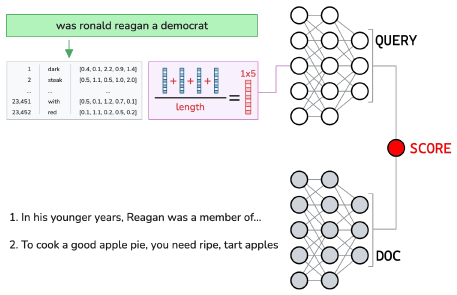
Two Towers

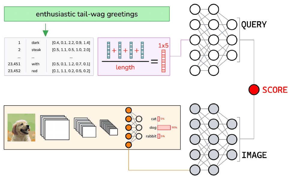
The two towers never see each other, and that constraint is what makes the design usable. The document tower never sees a query, so it can run before any query exists.

• Embed the whole corpus once, offline
• Put the vectors in an index
• At query time, embed one short string and look up its nearest neighbours

The alternative is one model reading the query and document together. It is more accurate. It also has to run once per document per query, which does not survive contact with a real corpus.

And because the towers only have to agree on a shared vector space, they do not have to be the same kind of model.

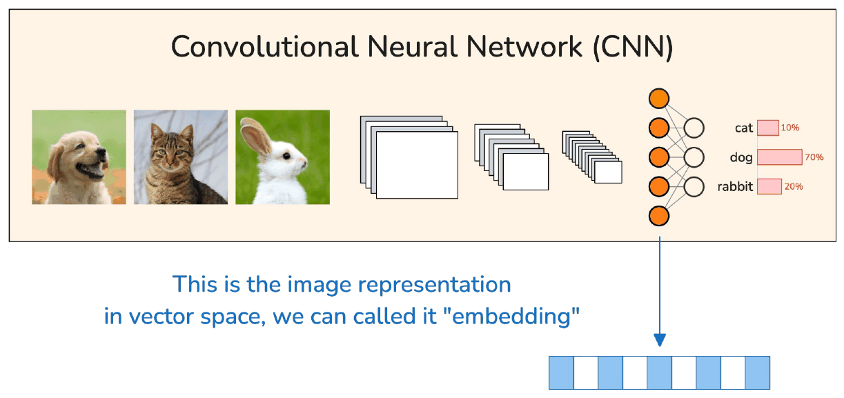
A CNN trained to classify images produces exactly the same kind of object partway through: a vector that summarises its input.

Swap the document tower for the image one and the architecture is unchanged. You can now search photographs with a sentence.

Nothing about the design had to be rethought. A piece of machinery gets reused for something it was not built for.

Building One

The rest of this page trains a small two-tower model, because the part that decides whether it works is not the architecture.

It needs query-document pairs, and MS MARCO is where they come from: real Bing queries, each with the passage a person marked as answering it. A query and its passage share almost no vocabulary, which is the case TF-IDF cannot handle and the reason for putting an encoder on each side.

# Setup, inlined rather than imported so this notebook runs on its own.
# Keep it folded; nothing below it depends on anything outside this file.

import torch.nn as nn
import visualtorch
import matplotlib.pyplot as plt

# --- chart styling -------------------------------------------------------
# Categorical slots of a CVD-validated palette: blue, orange, aqua, purple.
COLOURS = ["#2a78d6", "#eb6834", "#1baf7a", "#8a63d2"]
MUTED, GRID, AXIS = "#5b6570", "#e6e6e3", "#d5d5d1"


def style_axes(ax, xlabel=None, ylabel=None, grid="y"):
    """Strip an axes back to the ink that carries information."""
    if xlabel:
        ax.set_xlabel(xlabel, color=MUTED, fontsize=9)
    if ylabel:
        ax.set_ylabel(ylabel, color=MUTED, fontsize=9)
    if grid:
        ax.grid(axis=grid, color=GRID, linewidth=0.8)
        ax.set_axisbelow(True)
    for side in ("top", "right"):
        ax.spines[side].set_visible(False)
    for side in ("left", "bottom"):
        ax.spines[side].set_color(AXIS)
    ax.tick_params(colors=MUTED, labelsize=9, length=0)
    return ax


def figure(width=7.0, height=4.2, **kw):
    fig, ax = plt.subplots(figsize=(width, height), **kw)
    return fig, ax

# --- visualtorch, configured ---------------------------------------------
# Dropout is hidden: nn.TransformerEncoderLayer exposes its internal Dropout as a
# traceable leaf, every model here builds it with dropout=0.0, and drawing a no-op
# layer says it is part of the architecture when it is not. Uncoloured it also took
# visualtorch's default orange, near enough to MultiheadAttention's to be confusing.
COLOUR_MAP = {
    nn.Linear: {"fill": COLOURS[0]},
    nn.MultiheadAttention: {"fill": COLOURS[1]},
    nn.Embedding: {"fill": COLOURS[3]},
    nn.LayerNorm: {"fill": "#aeb6bf"},
    nn.GELU: {"fill": COLOURS[2]},
    nn.ReLU: {"fill": COLOURS[2]},
    nn.Flatten: {"fill": "#aeb6bf"},
    nn.Dropout: {"fill": "#e6e6e3"},
}
_COMMON = dict(color_map=COLOUR_MAP, connector_fill="#c3c9d0", background_fill="white",
               font_color=MUTED, legend=True, show_dimension=True,
               type_ignore=[nn.Dropout])


def diagram(model, input_shape, style="graph", **overrides):
    """Render `model` as a PIL image in this site's colours.

    `graph` draws real neurons and suits a short stack; `flow` draws volumetric
    blocks whose size tracks the layer's and stays readable on a deep one. `flow`
    reports a 3-D activation as (1, 1, width), losing the sequence length, so its
    shape labels are off. `level_gap=1` keeps a residual connection drawn close to
    the blocks it skips.
    """
    if style == "graph":
        settings = dict(node_size=24, layer_spacing=110, node_spacing=8,
                        ellipsize_after=5, **_COMMON)
    else:
        settings = dict(spacing=26, scale_xy=2.4, max_xy=280, one_dim_orientation="y",
                        level_gap=1, **_COMMON)
        settings["show_dimension"] = False
    settings.update(overrides)
    return visualtorch.render(model, input_shape=input_shape, style=style, **settings)


import collections
import re

import numpy as np
import torch
import torch.nn as nn
import torch.nn.functional as F
from datasets import load_dataset

DEVICE = torch.device("mps" if torch.backends.mps.is_available() else "cpu")

MARCO_REVISION = "a47ee7aae8d7d466ba15f9f0bfac3b3681087b3a"
marco = load_dataset("microsoft/ms_marco", "v1.1", split="train",
                     revision=MARCO_REVISION)

tokenise = lambda s: re.findall(r"[a-z0-9\+#]+", s.lower())

# A pair is a real query and the passage a person marked as answering it. Queries
# with no marked passage are dropped, since there is nothing to retrieve.
pairs = []
for row in marco:
    passages = row["passages"]
    answering = [text for text, selected
                 in zip(passages["passage_text"], passages["is_selected"]) if selected]
    if not answering:
        continue
    query, document = tokenise(row["query"]), tokenise(answering[0])
    if len(query) >= 3 and len(document) >= 8:
        pairs.append((query, document))

print(f"{len(pairs):,} query/document pairs from MS MARCO")
print(f"  query:    {' '.join(pairs[1][0])}")
print(f"  document: {' '.join(pairs[1][1])[:150]}...")

78,964 query/document pairs from MS MARCO
  query:    was ronald reagan a democrat
  document: from wikipedia the free encyclopedia a reagan democrat is a traditionally democratic voter in the united states especially a white working class north...

Real queries, and the passage a person marked as answering each one. The query has to find its passage out of every document held out, which is the whole task.

Query and passage each go through their own tower and come out as unit vectors. Recall@10 asks how often the right passage lands in the top ten of all five thousand, and chance is the number to hold it against.

EMBED, HIDDEN, MIN_COUNT = 128, 128, 2

# A vocabulary over the corpus, rather than hashing words into a fixed number of
# buckets, which collides two unrelated words into one row and makes the collision
# invisible.
counts = collections.Counter(w for query, document in pairs for w in query + document)
vocabulary = ["<pad>"] + [w for w, c in counts.most_common() if c >= MIN_COUNT]
word_id = {w: i for i, w in enumerate(vocabulary)}

# A query is a handful of words; a passage is a paragraph. They get their own
# lengths rather than one shared cap that would truncate every document.
QUERY_LEN, DOC_LEN = 24, 64


def encode(sequences, max_len):
    """Word ids, right-padded, with the true length alongside."""
    ids = torch.zeros(len(sequences), max_len, dtype=torch.long)
    lengths = torch.zeros(len(sequences), dtype=torch.long)
    for i, words in enumerate(sequences):
        kept = [word_id[w] for w in words if w in word_id][:max_len]
        ids[i, :len(kept)] = torch.tensor(kept, dtype=torch.long)
        lengths[i] = max(len(kept), 1)
    return ids, lengths


rng = np.random.default_rng(0)
order = rng.permutation(len(pairs))
held_out = 5_000
train_ids, test_ids = order[:-held_out], order[-held_out:]

Q, Q_len = encode([pairs[i][0] for i in train_ids], QUERY_LEN)
D, D_len = encode([pairs[i][1] for i in train_ids], DOC_LEN)
Q_test, Q_test_len = encode([pairs[i][0] for i in test_ids], QUERY_LEN)
D_test, D_test_len = encode([pairs[i][1] for i in test_ids], DOC_LEN)

Q, Q_len, D, D_len = Q.to(DEVICE), Q_len.to(DEVICE), D.to(DEVICE), D_len.to(DEVICE)
Q_test, Q_test_len = Q_test.to(DEVICE), Q_test_len.to(DEVICE)
D_test, D_test_len = D_test.to(DEVICE), D_test_len.to(DEVICE)


class Tower(nn.Module):
    """Word ids in, a unit vector out. The query and document sides get one each."""

    def __init__(self):
        super().__init__()
        self.embed = nn.Embedding(len(vocabulary), EMBED, padding_idx=0)
        self.net = nn.Sequential(nn.Linear(EMBED, HIDDEN), nn.ReLU(),
                                 nn.Linear(HIDDEN, HIDDEN))

    def forward(self, ids, lengths):
        # Mean over the real words. Padding is row zero and contributes nothing to
        # the sum, so dividing by the true length is the average over the words
        # that were actually there.
        pooled = self.embed(ids).sum(1) / lengths.clamp(min=1).unsqueeze(-1)
        return F.normalize(self.net(pooled), dim=-1)

def recall_at_10(query_tower, doc_tower):
    with torch.no_grad():
        similarity = query_tower(Q_test, Q_test_len) @ doc_tower(D_test, D_test_len).T
        top = similarity.topk(10, dim=1).indices
        answer = torch.arange(len(Q_test), device=DEVICE).unsqueeze(1)
        return (top == answer).any(1).float().mean().item()

CHANCE = 10 / len(D_test)
print(f"{len(vocabulary):,} words, {len(Q):,} training pairs, "
      f"{len(D_test):,} documents to search")
print(f"chance recall@10 = {CHANCE:.4f}")

68,176 words, 73,964 training pairs, 5,000 documents to search
chance recall@10 = 0.0020

Two in a thousand, then. That is what a model that has learned nothing scores, and every number below is worth reading against it.

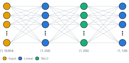
Drawn out, one tower is a stack of ordinary layers:

diagram(Tower(), input_shape=((1, DOC_LEN), (1,)),
        input_dtype=(torch.long, torch.long))

Figure 1: One tower. The query and document sides are each one of these, with separate weights, and the output is normalised so a dot product between two of them is a cosine.

Both towers start random, so their shared space means nothing yet. The training signal has to teach them what close means, and the obvious way is a triplet: a query, a document that answers it, and one that doesn’t. Pull the first pair together, push the second apart, by at least a margin.

def train(loss_fn, epochs=10, batch=256, seed=0):
    torch.manual_seed(seed)
    query_tower, doc_tower = Tower().to(DEVICE), Tower().to(DEVICE)
    optimiser = torch.optim.Adam([*query_tower.parameters(), *doc_tower.parameters()], lr=1e-3)
    generator = torch.Generator().manual_seed(seed)

    losses, recalls = [], []
    for _ in range(epochs):
        perm = torch.randperm(len(Q), generator=generator).to(DEVICE)
        total = steps = 0
        for i in range(0, len(perm) - batch, batch):
            b = perm[i:i + batch]
            loss = loss_fn(query_tower, doc_tower, b, perm, generator)
            optimiser.zero_grad()
            loss.backward()
            optimiser.step()
            total += loss.item()
            steps += 1
        losses.append(total / steps)
        recalls.append(recall_at_10(query_tower, doc_tower))
    return losses, recalls

MARGIN = 0.2

def triplet(query_tower, doc_tower, b, perm, generator):
    """One other document from the batch, picked at random, as the negative."""
    negatives = b[torch.randperm(len(b), generator=generator).to(DEVICE)]
    q = query_tower(Q[b], Q_len[b])
    positive = (q * doc_tower(D[b], D_len[b])).sum(-1)
    negative = (q * doc_tower(D[negatives], D_len[negatives])).sum(-1)
    return F.relu(MARGIN - positive + negative).mean()

triplet_loss, triplet_recall = train(triplet)
for epoch, (l, r) in enumerate(zip(triplet_loss, triplet_recall), 1):
    print(f"epoch {epoch}: loss {l:.4f}   recall@10 {r:.4f}   ({r / CHANCE:.1f}x chance)")

epoch 1: loss 0.1139   recall@10 0.0300   (15.0x chance)
epoch 2: loss 0.0781   recall@10 0.0364   (18.2x chance)
epoch 3: loss 0.0643   recall@10 0.0468   (23.4x chance)
epoch 4: loss 0.0534   recall@10 0.0554   (27.7x chance)
epoch 5: loss 0.0463   recall@10 0.0668   (33.4x chance)
epoch 6: loss 0.0402   recall@10 0.0716   (35.8x chance)
epoch 7: loss 0.0362   recall@10 0.0714   (35.7x chance)
epoch 8: loss 0.0324   recall@10 0.0846   (42.3x chance)
epoch 9: loss 0.0293   recall@10 0.0872   (43.6x chance)
epoch 10: loss 0.0262   recall@10 0.0932   (46.6x chance)

The loss falls steadily and recall climbs to forty-seven times chance, so the towers learn something. They learn it slowly, and the loss curve is much happier about the situation than the recall curve is.

A negative drawn at random is almost always about a completely different subject, so most of the time the towers only have to tell a question about tax from a question about knee surgery. They manage that early, the margin is satisfied, and a satisfied margin contributes no gradient. What is left to learn from is the small fraction of draws that happen to be hard, and that fraction shrinks as the model improves, so most of every batch stops teaching it anything while it is still unable to do the thing you actually want: pick the right passage out of thousands of plausible ones.

The standard fix is to use the whole batch. Every other document in it is a negative for this query, so each query is scored against hundreds of candidates rather than one, the hard ones are always in there somewhere, and the documents are already encoded.

TEMPERATURE = 0.05

def in_batch(query_tower, doc_tower, b, perm, generator):
    """Every other document in the batch is a negative for this query."""
    q, docs = query_tower(Q[b], Q_len[b]), doc_tower(D[b], D_len[b])
    return F.cross_entropy((q @ docs.T) / TEMPERATURE,
                           torch.arange(len(b), device=DEVICE))

batch_loss, batch_recall = train(in_batch)
for epoch, (l, r) in enumerate(zip(batch_loss, batch_recall), 1):
    print(f"epoch {epoch}: loss {l:.4f}   recall@10 {r:.4f}   ({r / CHANCE:.1f}x chance)")

epoch 1: loss 4.7703   recall@10 0.0658   (32.9x chance)
epoch 2: loss 3.9668   recall@10 0.1094   (54.7x chance)
epoch 3: loss 3.4015   recall@10 0.1420   (71.0x chance)
epoch 4: loss 2.9127   recall@10 0.1754   (87.7x chance)
epoch 5: loss 2.4703   recall@10 0.2012   (100.6x chance)
epoch 6: loss 2.0736   recall@10 0.2222   (111.1x chance)
epoch 7: loss 1.7290   recall@10 0.2442   (122.1x chance)
epoch 8: loss 1.4259   recall@10 0.2588   (129.4x chance)
epoch 9: loss 1.1743   recall@10 0.2738   (136.9x chance)
epoch 10: loss 0.9703   recall@10 0.2856   (142.8x chance)

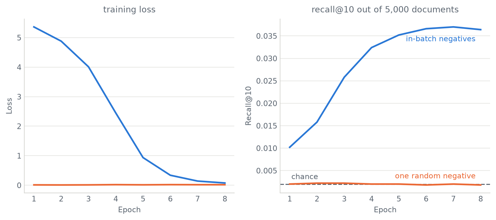
Recall passes where the triplet run finished by its second epoch and keeps going, ending at 143 times chance against its 47. Same towers, same data, same number of steps, and the only difference is where the negatives come from.

Both runs plotted together, loss on the left and recall on the right.

import matplotlib.pyplot as plt

epochs = range(1, len(batch_loss) + 1)
fig, (left, right) = plt.subplots(1, 2, figsize=(8.4, 3.8))

left.plot(epochs, triplet_loss, color=COLOURS[1], linewidth=2)
left.plot(epochs, batch_loss, color=COLOURS[0], linewidth=2)
left.set_title("training loss", fontsize=10, color=MUTED, pad=8)
style_axes(left, "Epoch", "Loss")

right.axhline(CHANCE, color=MUTED, linewidth=1.2, linestyle="--")
right.plot(epochs, triplet_recall, color=COLOURS[1], linewidth=2)
right.plot(epochs, batch_recall, color=COLOURS[0], linewidth=2)
right.annotate("in-batch negatives", xy=(epochs[-1], batch_recall[-1]), xytext=(-6, -14),
               textcoords="offset points", ha="right", fontsize=9, color=COLOURS[0])
right.annotate("one random negative", xy=(epochs[-1], triplet_recall[-1]), xytext=(-6, 8),
               textcoords="offset points", ha="right", fontsize=9, color=COLOURS[1])
right.annotate("chance", xy=(1, CHANCE), xytext=(2, 6), textcoords="offset points",
               fontsize=9, color=MUTED)
right.set_title("recall@10 out of 5,000 documents", fontsize=10, color=MUTED, pad=8)
style_axes(right, "Epoch", "Recall@10")
fig.tight_layout()

Figure 2: The same towers, the same data, the same number of steps. Only the choice of negatives differs.

Same towers, same data, same number of gradient steps. The triplet run even ends with the lower training loss. Rank the two runs by that number and you pick the worse model.

That is a category error rather than a paradox. The two losses are not the same quantity: one is a margin violation against a single negative, the other a cross-entropy over a few hundred. A loss is comparable to another loss on the same objective and to nothing else, which is why the right-hand panel carries a chance line and the left-hand one carries no verdict at all.

Conclusion

A search system comes in two halves.

• PageRank scores a document on its own merit, from the link graph
• A learned encoder scores whether it is about the right thing
• The encoder is the word2vec model, reused
• The same two-tower design works for images with no changes

The full project, with a Redis vector index, is on GitHub.