word2vec from Scratch: Turning the Meaning of Words into Numbers

Skip-gram and CBOW with negative sampling, written from scratch and trained on text8, then scored against WordSim-353, SimLex-999 and the Google analogy set.

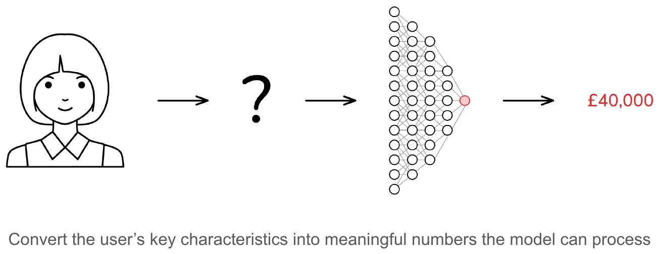
A neural network takes numbers in and gives a number out. Some of what you know about the world does not easily become a number.

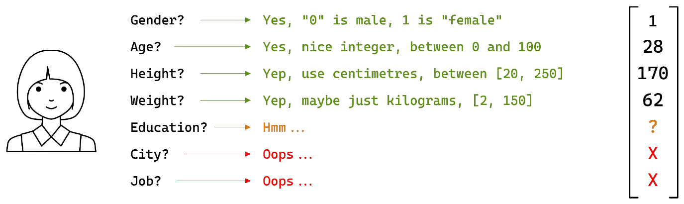
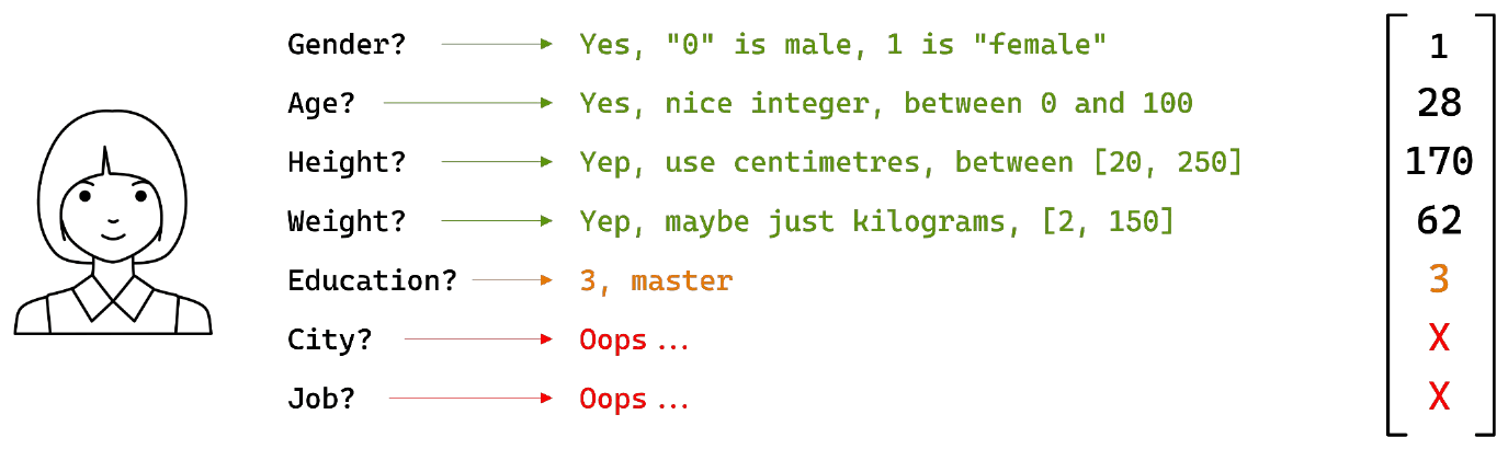
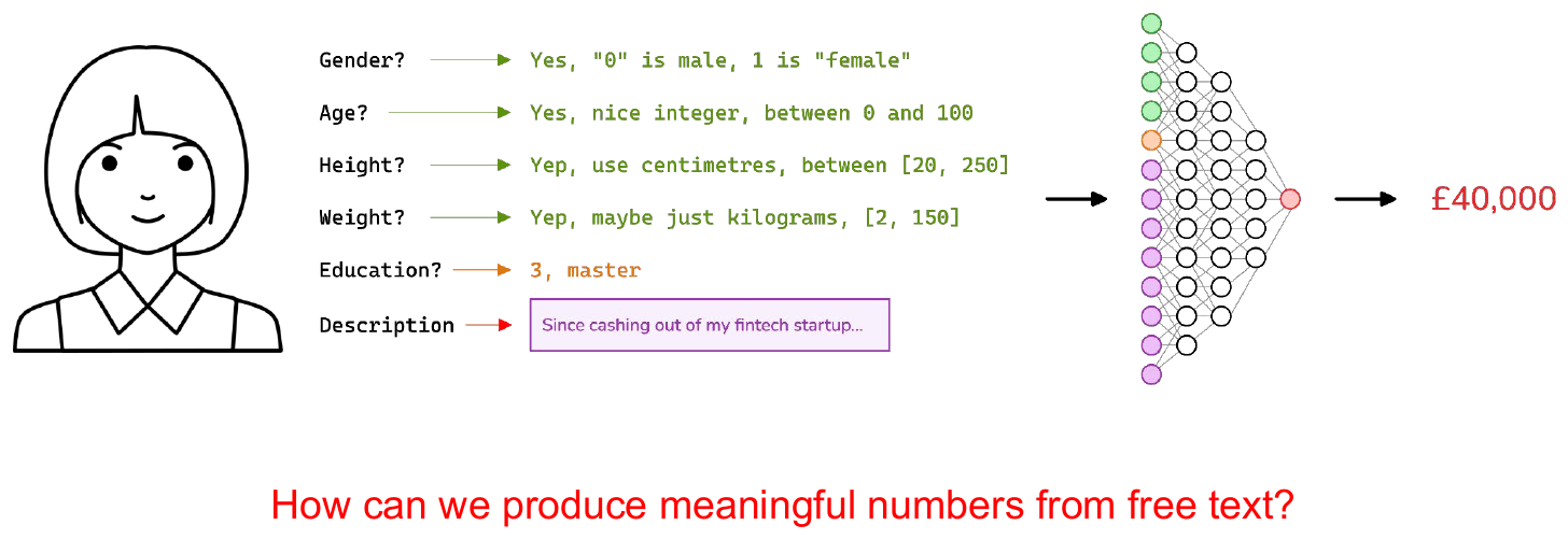
Predicting income from what a form records means turning each field on it into numbers the model can process.

Gender, age, height and weight each have an obvious numeric form. Education does not have one.

Feature Encoding

Education

Ordinal

One number per level, and it carries the ordering. It also tells the model that a PhD is four times a high school diploma, a ratio the levels do not have.

0 - none
1 - high-school
2 - bachelor
3 - master
4 - PhD

Years of Schooling

Still one number, and now the spacing between levels means something. But you had to know the answer. You supplied the domain knowledge, not the model.

0 - none
12 - high-school
15 - bachelor
17 - master
21 - PhD

One-Hot

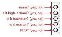
Five slots, one of them set to 1. It makes no claims about ordering or distance. The cost is a slot per category. It also makes every pair equally far apart, so a master’s and a PhD are as different as a PhD and no schooling.

[1, 0, 0, 0, 0] - none
[0, 1, 0, 0, 0] - high-school
[0, 0, 1, 0, 0] - bachelor
[0, 0, 0, 1, 0] - master
[0, 0, 0, 0, 1] - PhD

Learned Embeddings

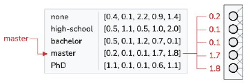
Five numbers per level, started at random and moved by training. No assumptions, no ordering imposed. The model decides what the numbers mean, at the cost of more parameters and the data needed to fit them.

[0.4, 0.1, 2.2, 0.9, 1.4] - none
[0.5, 1.1, 0.5, 1.0, 2.0] - high-school
[0.5, 0.1, 1.2, 0.7, 0.1] - bachelor
[0.2, 0.1, 0.1, 1.7, 1.8] - master
[1.1, 0.1, 0.1, 0.6, 1.1] - PhD

Learned embeddings are what the rest of this post builds. At this scale they look like overkill, because there are five categories and one-hot would do.

City

City has the same problem as education. No ordering, and a thousand categories instead of five. One-hot is now a thousand slots of mostly zeros.

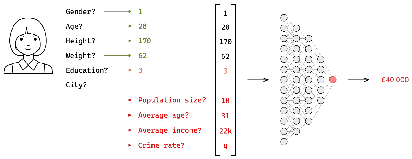
Break the category into features that describe it. A city is its population, its average age, its average income, its crime rate. Four numbers instead of a thousand. Each one means something. Two similar cities end up with similar numbers.

This is good feature engineering. A lot of real models are built this way. It also has a ceiling, and the next feature is above it.

Free Text

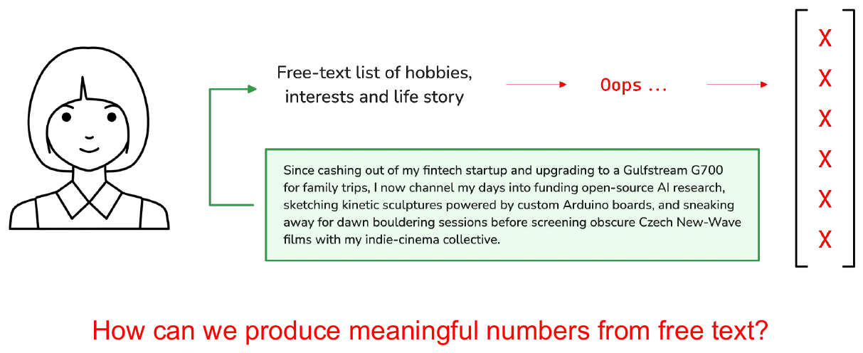
Now the form has a box that says tell us about yourself, filled in with a paragraph of prose, and there is no obvious way to turn that into numbers.

There is no decomposition to reach for. Cities have populations. Paragraphs do not have an agreed set of four numbers. The categories are unbounded, because the field accepts any text at all. Every trick used so far is gone.

How can we produce meaningful numbers from free text?

The Distributional Hypothesis

What is the meaning of bardiwac?

He handed her her glass of bardiwac.

Beef dishes are made to complement the bardiwacs.

Nigel staggered to his feet, face flushed from too much bardiwac.

I dined off bread and cheese and this excellent bardiwac.

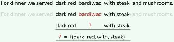
You have never seen that word before. After four sentences you know it is a drink. Probably a red wine. Probably alcoholic.

No definition was given. The meaning came from the company the word keeps.

This is the distributional hypothesis. A word can be described by the words that appear around it. If that holds, you can compute a word’s meaning from a large pile of ordinary text, and nothing has to be labelled.

The learned-embedding option is still the plan. What changed is that there is now a way to train it without labels.

The word2vec Recipe

Context Windows

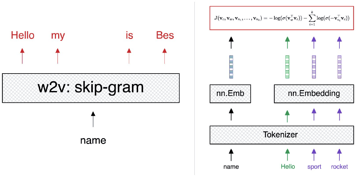
The window above is five tokens wide, so four neighbours predict the middle one. Width is a dial: the run here takes five words either side, which is what Mikolov et al. use and what the deployed service is configured with. That gives an enormous number of training examples from raw text, with no annotation.

The corpus is text8: the first 100MB of a Wikipedia dump, lowercased and stripped to letters and spaces.

# Setup, inlined rather than imported so this notebook runs on its own.
# Keep it folded; nothing below it depends on anything outside this file.

import matplotlib.pyplot as plt

# --- chart styling -------------------------------------------------------
# Categorical slots of a CVD-validated palette: blue, orange, aqua, purple.
COLOURS = ["#2a78d6", "#eb6834", "#1baf7a", "#8a63d2"]
MUTED, GRID, AXIS = "#5b6570", "#e6e6e3", "#d5d5d1"


def style_axes(ax, xlabel=None, ylabel=None, grid="y"):
    """Strip an axes back to the ink that carries information."""
    if xlabel:
        ax.set_xlabel(xlabel, color=MUTED, fontsize=9)
    if ylabel:
        ax.set_ylabel(ylabel, color=MUTED, fontsize=9)
    if grid:
        ax.grid(axis=grid, color=GRID, linewidth=0.8)
        ax.set_axisbelow(True)
    for side in ("top", "right"):
        ax.spines[side].set_visible(False)
    for side in ("left", "bottom"):
        ax.spines[side].set_color(AXIS)
    ax.tick_params(colors=MUTED, labelsize=9, length=0)
    return ax


def figure(width=7.0, height=4.2, **kw):
    fig, ax = plt.subplots(figsize=(width, height), **kw)
    return fig, ax


import collections

import numpy as np
import torch
import torch.nn.functional as F
from huggingface_hub import hf_hub_download

DEVICE = torch.device("mps" if torch.backends.mps.is_available() else "cpu")

# The project's settings, not a scaled-down version of them.
EMBED, WINDOW, NEGATIVES = 300, 5, 5
MIN_COUNT, SUBSAMPLE = 5, 1e-4
BATCH, LEARNING_RATE, EPOCHS, SEED = 4096, 1e-3, 10, 42

TEXT8 = "12fc5d108454e1d48dfba7e8ea4d2b0b10225291"
path = hf_hub_download("roshbeed/ai-residency-text8", "text8",
                       repo_type="dataset", revision=TEXT8)

words = open(path).read().split()
counts = collections.Counter(words)
vocab = [w for w, c in counts.most_common() if c >= MIN_COUNT]
stoi = {w: i for i, w in enumerate(vocab)}
ids = torch.tensor([stoi[w] for w in words if w in stoi], dtype=torch.int32)

print(f"{len(words):,} tokens, {len(counts):,} distinct, {len(vocab):,} kept")
print(f"'the' appears {counts['the']:,} times, "
      f"one word in {len(words) / counts['the']:.0f}")
print(f"training on {DEVICE}")

17,005,207 tokens, 253,854 distinct, 71,290 kept
'the' appears 1,061,396 times, one word in 16
training on mps

Seventeen million words, of which 71,290 distinct ones appear at least five times. Those are the words the model will learn a vector for.

One more step before training. the appears 1,061,396 times in that text, one word in sixteen, and it sits next to everything, so it tells you nothing about its neighbours. Common words get thrown away, and the more common a word is the more often it goes.

frequency = torch.bincount(ids.long(), minlength=len(vocab)).double()
frequency /= frequency.sum()

keep_probability = torch.clamp(torch.sqrt(torch.tensor(SUBSAMPLE) / frequency),
                               max=1.0).float()
noise = (frequency ** 0.75 / (frequency ** 0.75).sum()).float().to(DEVICE)

print(f"'the' survives with probability {keep_probability[stoi['the']]:.3f}, "
      f"'philosophy' with {keep_probability[stoi['philosophy']]:.3f}")

SPAN = 2 * WINDOW + 1


def windows(generator):
    """One epoch's worth of context windows, resampled each time.

    Subsampling is redrawn per epoch rather than once, so a frequent word is
    dropped from some passes and kept in others. `unfold` then gives every
    sliding window as a view, which costs nothing to build.
    """
    keep = torch.rand(len(ids), generator=generator) < keep_probability[ids.long()]
    return ids[keep].unfold(0, SPAN, 1)


sample = windows(torch.Generator().manual_seed(SEED))
print(f"{sample.shape[0]:,} windows per epoch, {SPAN} words wide")

'the' survives with probability 0.040, 'philosophy' with 0.779
8,430,294 windows per epoch, 11 words wide

So the survives four times in a hundred, and philosophy about four times in five. Pairing each surviving word with the five words either side of it gives ten pairs per word, and those pairs are what the model trains on.

Negative Sampling

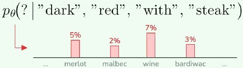
“For dinner we served dark red ___ with steak” does not have one right answer. It could be bardiwac, wine, merlot or malbec, so the model is not trained to output one word. It is trained to output a score for every word in the vocabulary, and words that fit the same gaps end up with similar scores, which pulls their vectors together.

Scoring every word is expensive. To turn raw scores into probabilities you need a softmax: exponentiate each score, then divide by the total so they add up to one. The total is over the whole vocabulary, 71,290 words here, so every training step touches all of them to learn one thing.

Negative sampling changes the question. Instead of asking which of these 71,290 words goes here, it asks is this pair real, or did I make it up. Once for the true neighbour, then five more times for words picked at random: six comparisons instead of 71,290.

Where the random words come from matters:

• Pick uniformly and nearly every one is a rare word the model already scores near zero. It learns nothing.
• Pick by raw frequency and nearly all of them are the.
• Mikolov et al. raise the frequencies to the power 3/4, which sits between the two.

The loss is that question asked in code: true pairs pushed up, invented ones pushed down. How many of each depends on which way round you predict, which is what CBOW and skip-gram differ on.

def loss_on(rows, inside, outside, architecture, generator):
    """Score the real pairs up and the invented ones down.

    skip-gram takes the centre vector and predicts each of the 2*WINDOW context
    words, so it scores 2*WINDOW positives and NEGATIVES invented words for each.
    CBOW averages the context into one vector and predicts the centre, so it
    scores one positive and NEGATIVES invented words.
    """
    rows = rows.to(DEVICE).long()
    centre = rows[:, WINDOW]
    context = torch.cat((rows[:, :WINDOW], rows[:, WINDOW + 1:]), dim=1)
    batch = rows.shape[0]

    if architecture == "skipgram":
        vector = inside[centre].unsqueeze(1)
        real = F.logsigmoid((vector * outside[context]).sum(-1)).sum(-1)
        drawn = 2 * WINDOW * NEGATIVES
    else:
        vector = inside[context].mean(1).unsqueeze(1)
        real = F.logsigmoid((vector.squeeze(1) * outside[centre]).sum(-1))
        drawn = NEGATIVES

    invented_ids = torch.multinomial(noise, batch * drawn, replacement=True,
                                     generator=generator)
    invented = outside[invented_ids.view(batch, drawn)]
    fake = F.logsigmoid(-(invented @ vector.squeeze(1).unsqueeze(-1)).squeeze(-1)).sum(-1)
    return -(real + fake).mean()

CBOW and Skip-gram

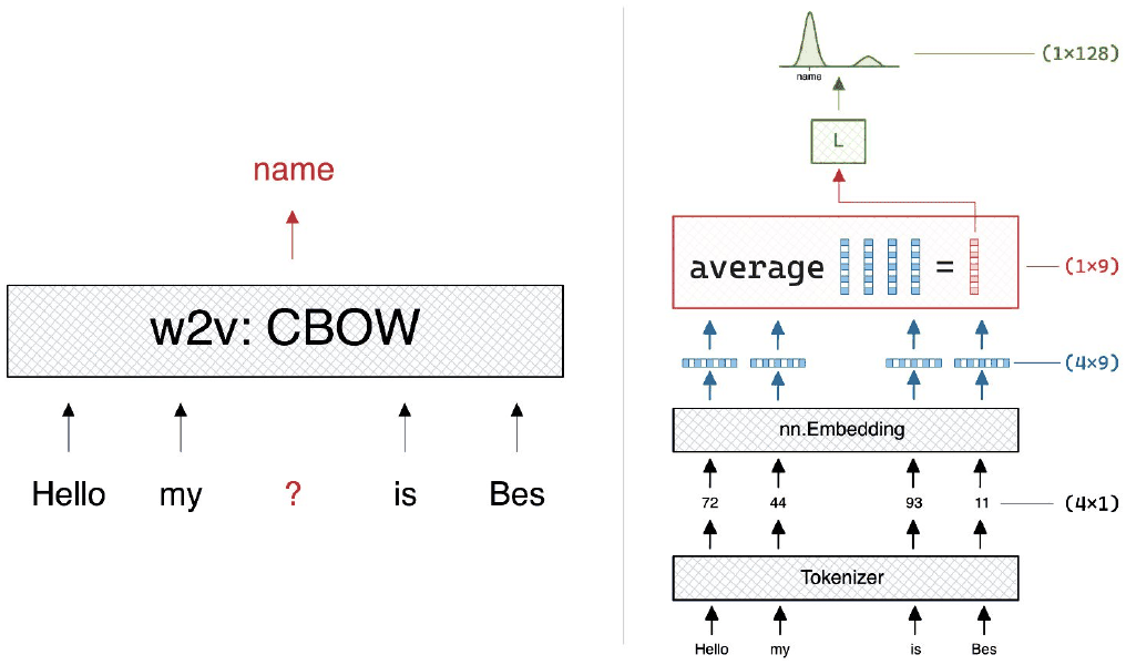
There are two ways to arrange that prediction.

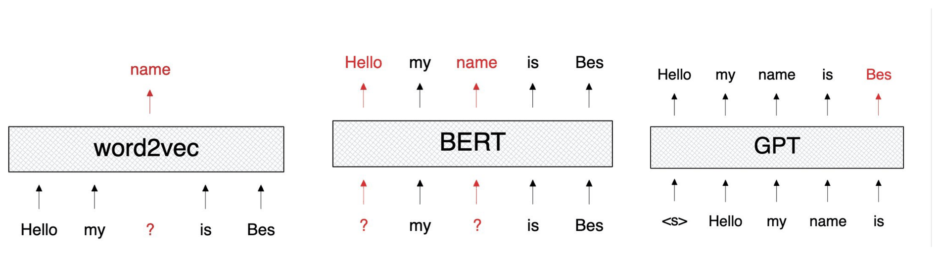
CBOW takes the context and predicts the middle word.

Skip-gram runs it the other way. One word in, predict each of its neighbours.

Either way there are two tables of vectors. One holds a word’s vector when it’s the centre of a window. The other holds it when it appears in another word’s context. Only the first is kept at the end; the second exists to give the first something to be scored against.

Skip-gram scores ten true pairs per window, one for each context word, where CBOW averages the context and scores one, so the two start from different losses.

def new_model(generator):
    """Two matrices. The first is the one you keep."""
    inside = (torch.randn(len(vocab), EMBED, generator=generator) * 0.01)
    # Small random, not zeros. Zeros force every dot product to 0, which would make
    # the baseline below exactly (positives + negatives) * ln 2 by construction
    # rather than by measurement.
    outside = (torch.randn(len(vocab), EMBED, generator=generator) * 0.01)
    return inside.to(DEVICE).requires_grad_(), outside.to(DEVICE).requires_grad_()


# A model that knows nothing is guessing on every pair it scores, and each costs
# ln 2. That is a different number for each architecture, which is the point.
for architecture, terms in (("skipgram", 2 * WINDOW * (1 + NEGATIVES)),
                            ("cbow", 1 + NEGATIVES)):
    generator = torch.Generator(device=DEVICE).manual_seed(SEED)
    inside, outside = new_model(torch.Generator().manual_seed(SEED))
    with torch.no_grad():
        measured = loss_on(sample[:BATCH], inside, outside, architecture, generator).item()
    print(f"{architecture:9} loss before training: {measured:7.3f}, "
          f"and {terms} * ln 2 = {terms * np.log(2):7.3f}")

skipgram  loss before training:  41.589, and 60 * ln 2 =  41.589
cbow      loss before training:   4.159, and 6 * ln 2 =   4.159

Those numbers matching is a useful check. A model that knows nothing is guessing on every pair it scores, and each guess costs ln 2. Skip-gram scores sixty pairs per window — ten real and fifty invented — so it starts at sixty times ln 2. CBOW scores six. Both land on their own figure to three decimals.

What it catches is the arithmetic around the loss: that there really are K negatives and not three, that they are summed while the batch is averaged, that nothing is double-counted. It does not catch a sign error. At initialisation the vectors are near zero, so every dot product is near zero, and sigmoid is a half either way. Flip the minus in front of the invented pairs and this line still prints 41.589.

Ten passes over the corpus, once for each architecture.

embeddings = {}
history = {}

for architecture in ("skipgram", "cbow"):
    cpu_generator = torch.Generator().manual_seed(SEED)
    gpu_generator = torch.Generator(device=DEVICE).manual_seed(SEED)
    inside, outside = new_model(torch.Generator().manual_seed(SEED))
    optimiser = torch.optim.Adam([inside, outside], lr=LEARNING_RATE)

    losses = []
    for epoch in range(EPOCHS):
        rows = windows(cpu_generator)
        order = torch.randperm(rows.shape[0], generator=cpu_generator)
        total = steps = 0
        for start in range(0, rows.shape[0] - BATCH, BATCH):
            loss = loss_on(rows[order[start:start + BATCH]], inside, outside,
                           architecture, gpu_generator)
            optimiser.zero_grad()
            loss.backward()
            optimiser.step()
            total += loss.item()
            steps += 1
        losses.append(total / steps)

    embeddings[architecture] = inside.detach()
    history[architecture] = losses
    print(f"{architecture:9} {losses[0]:7.3f} -> {losses[-1]:7.3f} "
          f"over {EPOCHS} epochs")

skipgram   25.731 ->  20.867 over 10 epochs
cbow        2.487 ->   1.351 over 10 epochs

Down from each architecture’s own coin baseline, which is the only thing either number means on its own. What the training bought shows up in the vectors rather than in the loss: cosine similarity between them gives the words nearest any word in the vocabulary.

space = F.normalize(embeddings["skipgram"], dim=1)


def nearest(word, k=6):
    similarity = space @ space[stoi[word]]
    similarity[stoi[word]] = -1
    return [vocab[i] for i in similarity.topk(k).indices.tolist()]


for word in ("king", "france", "computer", "three", "war", "music"):
    print(f"{word:10} {', '.join(nearest(word))}")

king       crowned, kings, throne, reigned, anshan, ethelwulf
france     french, germany, belgium, spain, paris, philippe
computer   computers, hardware, computing, software, microcomputer, graphics
three      four, two, one, five, six, seven
war        civil, wwii, hostilities, battle, corregidor, ii
music      musical, musicians, folk, melodic, danceable, allmusic

Nothing labelled any of that. The lists come out of counting which words turn up near which.

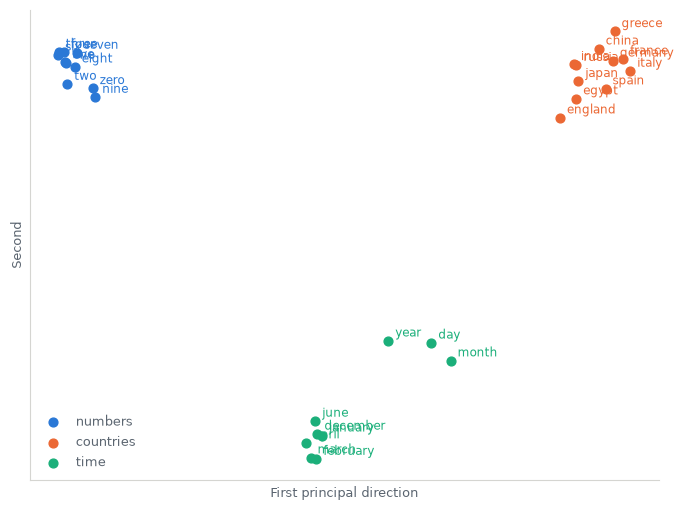
Three hundred numbers per word is more than can be drawn, so the last step is to flatten them onto a plane. Take three groups of words that have nothing in common except their category, find the two directions that separate them most, and plot only those.

import matplotlib.pyplot as plt

GROUPS = {
    "numbers": ["one", "two", "three", "four", "five", "six", "seven", "eight",
                "nine", "zero"],
    "countries": ["france", "germany", "italy", "spain", "russia", "china", "japan",
                  "england", "greece", "egypt", "india"],
    "time": ["january", "february", "march", "april", "june", "december", "year",
             "day", "month"],
}
present = {name: [w for w in words if w in stoi] for name, words in GROUPS.items()}
picked = [w for words in present.values() for w in words]

# Principal components of just these words: the two directions along which this
# particular set of thirty spreads out most. Not a general map of the space.
M = space[[stoi[w] for w in picked]].cpu().numpy()
M = M - M.mean(0)
xy = M @ np.linalg.svd(M, full_matrices=False)[2][:2].T

fig, ax = figure(width=7.0, height=5.2)
start = 0
for (name, words), colour in zip(present.items(), COLOURS):
    points = xy[start:start + len(words)]
    ax.scatter(points[:, 0], points[:, 1], s=40, color=colour, zorder=3, label=name)
    for word, (x, y) in zip(words, points):
        ax.annotate(word, (x, y), xytext=(5, 3), textcoords="offset points",
                    fontsize=8.5, color=colour)
    start += len(words)

ax.legend(frameon=False, fontsize=9, labelcolor=MUTED, loc="best")
style_axes(ax, "First principal direction", "Second", grid=None)
ax.set_xticks([])
ax.set_yticks([])
fig.tight_layout()

Figure 1: Thirty words from three categories, projected onto the two directions that spread them furthest apart. Nothing in training was told these categories exist.

Three groups in three regions. Every word now has 300 numbers attached, and the numbers put related words near each other. Nothing was labelled to make it happen.

The number words are packed so tightly their labels sit on top of each other, because three and four and seven turn up in almost identical company. The time group splits again inside itself, the six month names in one knot and year, day and month off to one side, so the distances carry information as well as the clusters.

To turn a paragraph into numbers, look up each word and average. Crude, and enough to close the loop we opened with:

The free-text box goes in. Every feature on that form is now a number.

Evals

Three standard benchmarks, scored against the numbers the negative-sampling paper reported on this same corpus.

from scipy.stats import spearmanr

EVAL = "80a775cc6dc61771da6ff6ea21f5703ae665a2e2"
benchmark_file = {
    name: hf_hub_download("roshbeed/ai-residency-word-embeddings-eval", name,
                          repo_type="dataset", revision=EVAL)
    for name in ("wordsim353.txt", "simlex999.txt", "questions-words.txt")
}


def similarity(vectors, path):
    """Spearman between cosine similarity and the benchmark score."""
    rows = [line.split() for line in open(path, encoding="utf-8").read().splitlines()]
    pairs = [(r[0].lower(), r[1].lower(), float(r[2])) for r in rows if len(r) == 3]
    usable = [(stoi[a], stoi[b], s) for a, b, s in pairs if a in stoi and b in stoi]
    unit = F.normalize(vectors, dim=1)
    left = unit[torch.tensor([u[0] for u in usable], device=vectors.device)]
    right = unit[torch.tensor([u[1] for u in usable], device=vectors.device)]
    predicted = (left * right).sum(1).cpu().tolist()
    return float(spearmanr(predicted, [u[2] for u in usable])[0]), len(usable) / len(pairs)


def analogies(vectors, path, max_vocab=30_000):
    """`a is to b as c is to ?`, answered over the most frequent words only."""
    questions, semantic = [], True
    for line in open(path, encoding="utf-8").read().splitlines():
        if line.startswith(":"):
            semantic = not line.split()[1].startswith("gram")
            continue
        fields = line.lower().split()
        if len(fields) == 4:
            questions.append((*fields, semantic))

    candidates = min(max_vocab, vectors.shape[0])
    unit = F.normalize(vectors[:candidates], dim=1)
    usable = [tuple(stoi[w] for w in q[:4]) for q in questions
              if all(w in stoi and stoi[w] < candidates for w in q[:4])]

    correct = 0
    for start in range(0, len(usable), 512):
        chunk = torch.tensor(usable[start:start + 512], device=vectors.device)
        query = F.normalize(unit[chunk[:, 1]] - unit[chunk[:, 0]] + unit[chunk[:, 2]], dim=1)
        scores = query @ unit.T
        # a, b and c are excluded, not merely deprioritised: the query vector is a
        # short hop from c, so without this the answer is almost always c itself.
        scores.scatter_(1, chunk[:, :3], float("-inf"))
        correct += (scores.argmax(1) == chunk[:, 3]).sum().item()
    return correct / len(usable), len(usable) / len(questions)


untrained, _ = new_model(torch.Generator().manual_seed(SEED))
scored = {"untrained": untrained.detach(), **embeddings}

print(f"{'':20}" + "".join(f"{name:>12}" for name in scored) + "  published  coverage")
for label, scorer, published in (
        ("WordSim-353", lambda v: similarity(v, benchmark_file["wordsim353.txt"]), 0.68),
        ("SimLex-999", lambda v: similarity(v, benchmark_file["simlex999.txt"]), 0.30),
        ("Google analogies", lambda v: analogies(v, benchmark_file["questions-words.txt"]), 0.38)):
    values, coverage = [], 0.0
    for vectors in scored.values():
        score, coverage = scorer(vectors)
        values.append(score)
    print(f"{label:20}" + "".join(f"{v:12.3f}" for v in values)
          + f"{published:11.2f}{coverage:10.2f}")

                       untrained    skipgram        cbow  published  coverage
WordSim-353                0.063       0.733       0.741       0.68      0.99
SimLex-999                -0.001       0.316       0.308       0.30      0.99
Google analogies           0.000       0.460       0.444       0.38      0.63

All three beat the published numbers for word2vec on this corpus. The untrained column is why that is worth stating: the same matrices before a single gradient step score 0.063, -0.001 and 0.000.

Vector Arithmetic

The famous claim is that directions in this space mean something. Take king, subtract man, add woman, and you should land near queen. Three more of the same shape, and the rank queen actually gets.

def analogy(a, b, c, k=3):
    """b is to a as ? is to c, with all three query words excluded."""
    query = F.normalize(space[stoi[b]] - space[stoi[a]] + space[stoi[c]], dim=0)
    scores = space @ query
    scores[[stoi[a], stoi[b], stoi[c]]] = float("-inf")
    order = scores.argsort(descending=True)
    return [vocab[i] for i in order[:k].tolist()], order


for a, b, c in (("big", "bigger", "small"), ("walk", "walked", "run"),
                ("france", "paris", "italy"), ("man", "king", "woman")):
    top, _ = analogy(a, b, c)
    print(f"{b} - {a} + {c:8} -> {', '.join(top)}")

_, order = analogy("man", "king", "woman")
rank = (order == stoi["queen"]).nonzero().item() + 1
print(f"\nqueen is ranked {rank} for king - man + woman")

family = [("man", "woman", "king", "queen"), ("father", "mother", "son", "daughter"),
          ("boy", "girl", "brother", "sister"), ("father", "mother", "grandfather",
          "grandmother"), ("husband", "wife", "brother", "sister")]
hits = sum(analogy(a, b, c, k=1)[0][0] == d for a, b, c, d in family
           if all(w in stoi for w in (a, b, c, d)))
print(f"{hits} of {len(family)} family analogies land first")

bigger - big + small    -> large, smaller, larger
walked - walk + run      -> runs, unearned, running
paris - france + italy    -> bologna, turin, venice
king - man + woman    -> queen, crowned, reigned

queen is ranked 1 for king - man + woman
3 of 5 family analogies land first

queen comes first. That is the result the claim promises, and this corpus has a reputation for not giving it.

The three that look easier are the ones that miss. walked - walk + run puts runs and running at the top and never reaches ran. paris - france + italy gives bologna, turin and venice: Italian cities, the right region of the space, the wrong city. bigger - big + small finds smaller second rather than first.

So the directions are there and reading one exact word off them is closer to a coin flip. The Google set scores 0.460 for the same reason — the arithmetic points the right way far more often than it lands on the intended word. Three of the five family analogies come first, which is the same story from the other side.

This text is 17 million words of Wikipedia, and king appears mostly in lists of monarchs and succession prose. The gender direction survives that; the precision does not.

Conclusion

The same model on a real dataset is predicting Hacker News upvotes: how many upvotes a post gets, from its title, its timestamp, its link and its author. A number to predict, some easy features, and one free-text field. These vectors fill that field in.

The window that makes this work is also what limits it. CBOW and skip-gram only ever see five words either side. Replace that fixed window with attention over the whole sequence and you get BERT and GPT, which is where the vision transformer picks up.

The full project, with the sweep and the deployed API, is on GitHub.