What attention does, why the architecture is called a transformer, and what the position embeddings are worth once the patches are in place.
Author
Rosh Beed
Published
June 22, 2026
Why is it called a transformer?
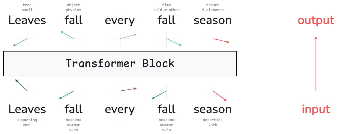
Leaves fall every fall season.
Going in, every word is ambiguous. Leaves could be foliage or departing. Fall could be the season or the verb, and it appears twice meaning different things.
A word2vec embedding gives each word one vector. That single vector has to cover every sense of the word. fall gets the same numbers whether it means autumn or dropping.
Coming out, each word has one meaning. The block has rewritten each word’s vector using the other words present. That’s its job. It transforms a representation of a word into a representation of that word in this context.
Attention
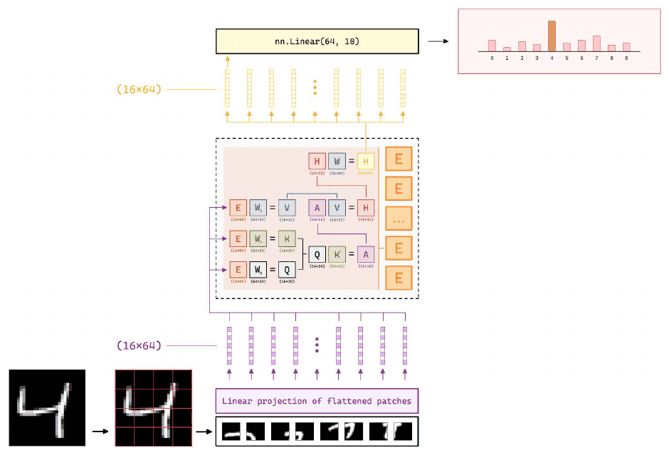
Each token produces three vectors. A query, which is what it is looking for. A key, which is what it offers. A value, which is what it passes on if chosen.
Every token’s query is compared against every token’s key by dot product, giving a score for each pair. Those scores go through a softmax, which exponentiates them and divides by the total so they become weights adding up to one. Each token’s new representation is then the weighted sum of everyone’s values.
If that sounds like a lookup table with fuzzy keys, that is roughly right. The difference is that nothing is looked up exactly; every token contributes a little, in proportion to how well its key matched.
fall asks “am I near a season word or a motion word”, season answers, and fall’s vector moves accordingly.
The Square Root
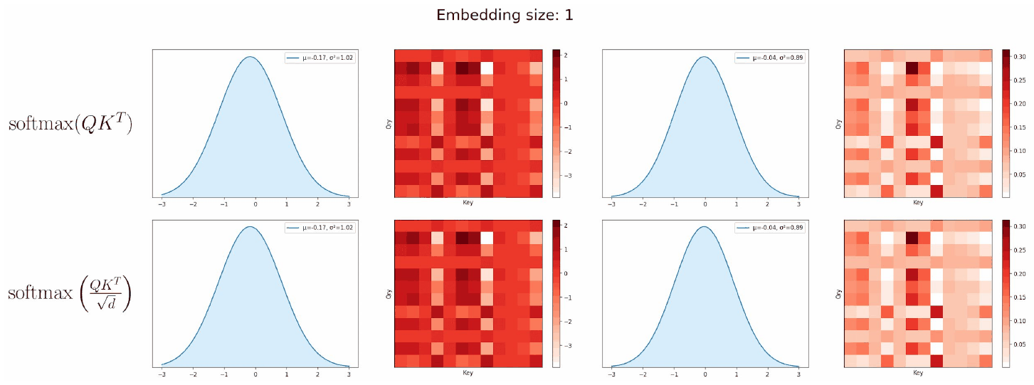
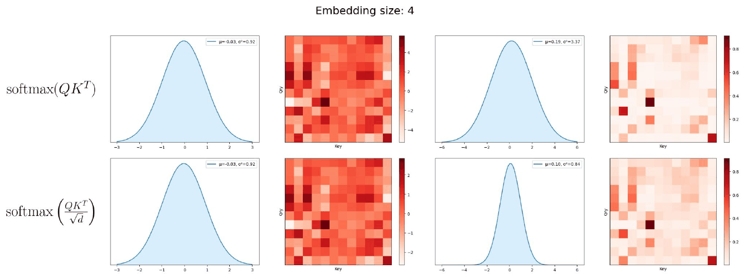
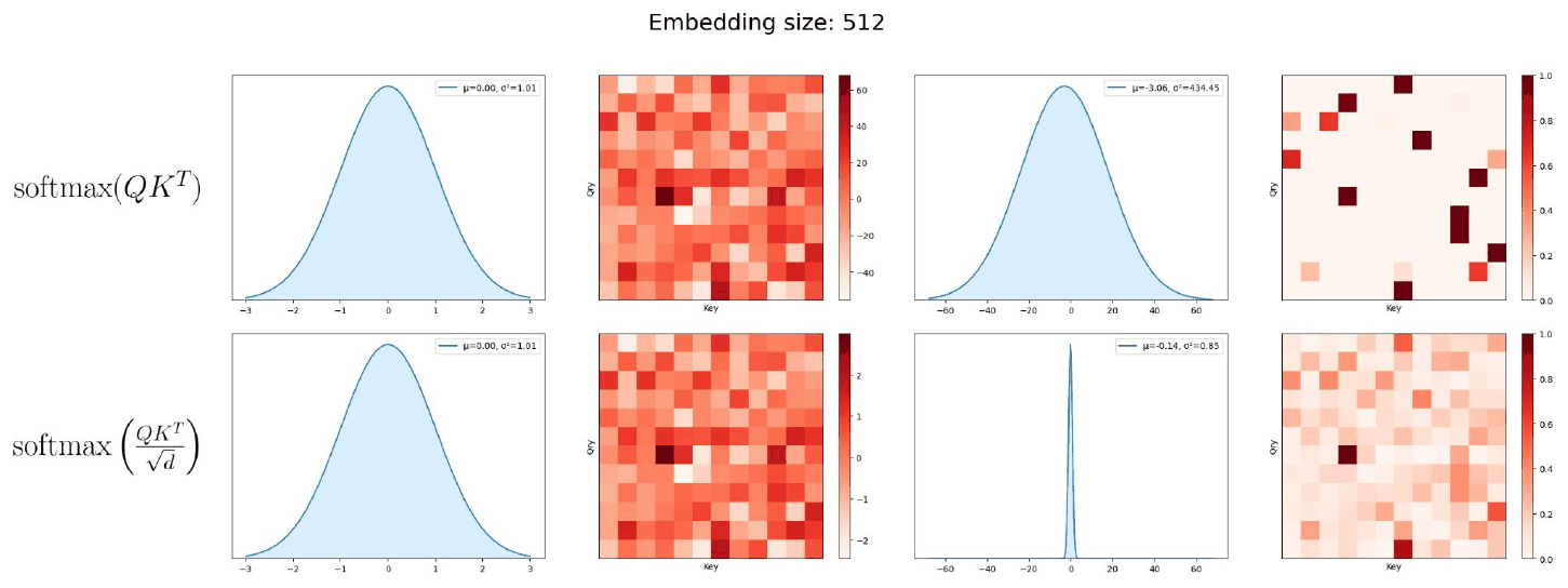
That denominator, \(\sqrt{d_k}\), looks like a detail. It is not, and the workshop showed why rather than asserting it: the same attention computed at three embedding sizes, with and without the scaling.
At one dimension there is nothing to choose between them.
At four, the unscaled scores are spreading out.
At 512 the unscaled version has fallen over. A dot product sums one term per dimension, so with 512 dimensions the scores are simply bigger numbers. Exponentiate bigger numbers and the largest one dominates completely. Almost all the weight lands on a single token and everything else gets close to nothing.
Attention stops being a weighted average and becomes a hard lookup. Worse, a weight pinned at zero or one barely responds to small changes in the inputs, so the model stops being able to learn from it.
Dividing by \(\sqrt{d_k}\) keeps the scores in the range where softmax is still soft. It is one symbol in the formula and it is the difference between the mechanism working and not.
The Task
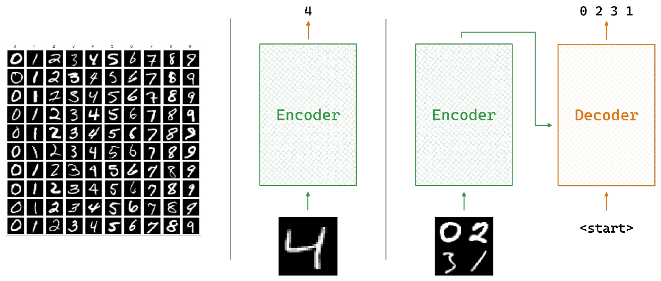
This is both halves of that diagram. Recognise one digit with an encoder, then read a multi-digit number with an encoder and a decoder. This post is the left-hand side; the next one is the right.
A picture is worth a thousand words. Can you write them?
The awkward part is that a transformer eats a sequence of tokens. An image is not one. It is a grid of pixels with no natural order, and there are far too many of them.
Attention compares every position with every other. Cost grows with the square of the sequence length. A 28×28 digit is 784 positions. A photograph is hopeless.
Patches
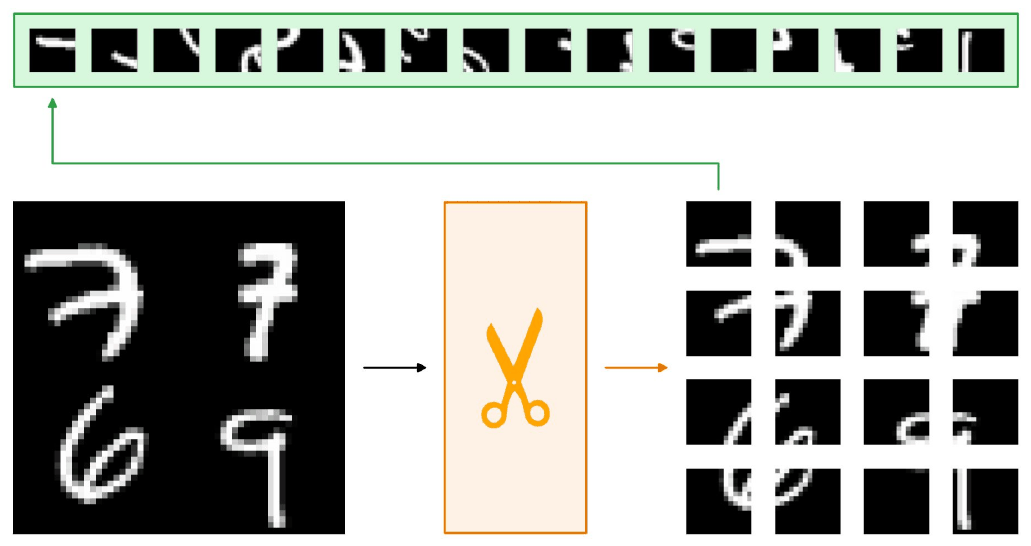
The Vision Transformer’s answer is to stop treating pixels as the unit. Cut the image into fixed-size squares and treat each square as a word.
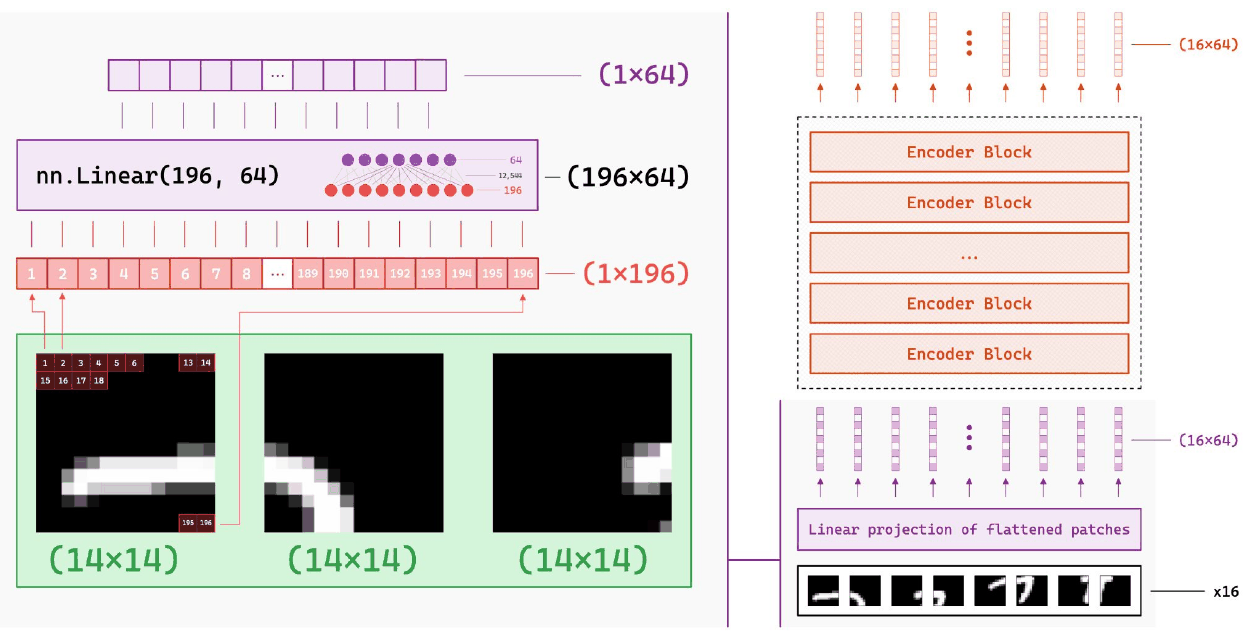
Flattening each patch through one Linear layer is the entire modification.
A 196-pixel patch becomes a 64-number vector. A word became a 64-number vector in word2vec. The transformer reading them cannot tell the difference.
One Encoder, Any Input
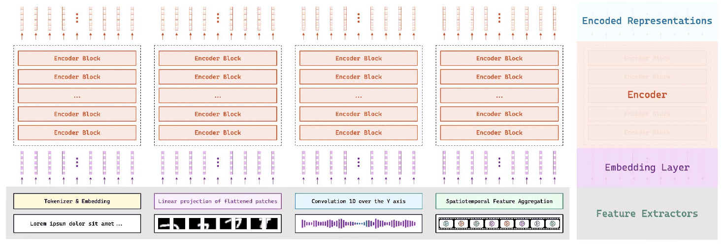
This is the diagram that makes it worth more than a digit classifier.
Text goes through a tokenizer and an embedding table. An image goes through a linear projection of flattened patches. Audio goes through a 1-D convolution over frequency. They all produce the same thing: a sequence of vectors.
Everything after that is identical. The encoder does not know what modality it is reading. Which means the work of supporting a new input type is writing a new front-end, not designing a new model.
Building One
What follows is that architecture shrunk until it trains when this page is run: 7×7 patches, two encoder layers, 64 dimensions, six thousand digits. The real service uses 4×4 patches into 128 dimensions, six layers and eight heads, with the attention and encoder blocks written out by hand rather than taken from PyTorch.
Position embeddings here are learned rather than sinusoidal, so they can be deleted to see what they were holding up.
First the digits, cut into patches. The number to keep hold of is the last one: what you score by ignoring the image and always guessing the most common digit.
Show the code
# Setup, inlined rather than imported so this notebook runs on its own.# Keep it folded; nothing below it depends on anything outside this file.import torch.nn as nnimport visualtorchimport matplotlib.pyplot as plt# --- chart styling -------------------------------------------------------# Categorical slots of a CVD-validated palette: blue, orange, aqua, purple.COLOURS = ["#2a78d6", "#eb6834", "#1baf7a", "#8a63d2"]MUTED, GRID, AXIS ="#5b6570", "#e6e6e3", "#d5d5d1"def style_axes(ax, xlabel=None, ylabel=None, grid="y"):"""Strip an axes back to the ink that carries information."""if xlabel: ax.set_xlabel(xlabel, color=MUTED, fontsize=9)if ylabel: ax.set_ylabel(ylabel, color=MUTED, fontsize=9)if grid: ax.grid(axis=grid, color=GRID, linewidth=0.8) ax.set_axisbelow(True)for side in ("top", "right"): ax.spines[side].set_visible(False)for side in ("left", "bottom"): ax.spines[side].set_color(AXIS) ax.tick_params(colors=MUTED, labelsize=9, length=0)return axdef figure(width=7.0, height=4.2, **kw): fig, ax = plt.subplots(figsize=(width, height), **kw)return fig, ax# --- visualtorch, configured ---------------------------------------------# Dropout is hidden: nn.TransformerEncoderLayer exposes its internal Dropout as a# traceable leaf, every model here builds it with dropout=0.0, and drawing a no-op# layer says it is part of the architecture when it is not. Uncoloured it also took# visualtorch's default orange, near enough to MultiheadAttention's to be confusing.COLOUR_MAP = { nn.Linear: {"fill": COLOURS[0]}, nn.MultiheadAttention: {"fill": COLOURS[1]}, nn.Embedding: {"fill": COLOURS[3]}, nn.LayerNorm: {"fill": "#aeb6bf"}, nn.GELU: {"fill": COLOURS[2]}, nn.ReLU: {"fill": COLOURS[2]}, nn.Flatten: {"fill": "#aeb6bf"}, nn.Dropout: {"fill": "#e6e6e3"},}_COMMON =dict(color_map=COLOUR_MAP, connector_fill="#c3c9d0", background_fill="white", font_color=MUTED, legend=True, show_dimension=True, type_ignore=[nn.Dropout])def diagram(model, input_shape, style="graph", **overrides):"""Render `model` as a PIL image in this site's colours. `graph` draws real neurons and suits a short stack; `flow` draws volumetric blocks whose size tracks the layer's and stays readable on a deep one. `flow` reports a 3-D activation as (1, 1, width), losing the sequence length, so its shape labels are off. `level_gap=1` keeps a residual connection drawn close to the blocks it skips. """if style =="graph": settings =dict(node_size=24, layer_spacing=110, node_spacing=8, ellipsize_after=5, **_COMMON)else: settings =dict(spacing=26, scale_xy=2.4, max_xy=280, one_dim_orientation="y", level_gap=1, **_COMMON) settings["show_dimension"] =False settings.update(overrides)return visualtorch.render(model, input_shape=input_shape, style=style, **settings)import numpy as npimport torchimport torch.nn as nnfrom huggingface_hub import hf_hub_downloadDEVICE = torch.device("mps"if torch.backends.mps.is_available() else"cpu")REVISION ="6bbb59474efaf5edfb62408686909305dbd45335"data = np.load(hf_hub_download("roshbeed/ai-residency-blog-data", "mnist/mnist-full.npz", repo_type="dataset", revision=REVISION))images = torch.from_numpy(data["x_train"]).float().div(255.0)labels = torch.from_numpy(data["y_train"]).long()# The service holds out a fifth of the training set to decide when to stop, so the# test set is never used to choose a model, only to report one.split =int(0.8*len(images))x_train, y_train = images[:split].to(DEVICE), labels[:split].to(DEVICE)x_val, y_val = images[split:].to(DEVICE), labels[split:].to(DEVICE)x_test = torch.from_numpy(data["x_test"]).float().div(255.0).to(DEVICE)y_test = torch.from_numpy(data["y_test"]).long().to(DEVICE)PATCH =4PATCHES = (28// PATCH) **2def patchify(images):"""28x28 -> 16 patches of 7x7, flattened. This is the whole trick.""" batch = images.shape[0] tiles = images.unfold(1, PATCH, PATCH).unfold(2, PATCH, PATCH)return tiles.reshape(batch, PATCHES, PATCH * PATCH)baseline = torch.bincount(y_test.cpu()).max().item() /len(y_test)print(f"{len(x_train):,} training digits, each becoming {PATCHES} tokens of {PATCH * PATCH}")print(f"always guessing the most common digit: {baseline:.4f}")
48,000 training digits, each becoming 49 tokens of 16
always guessing the most common digit: 0.1135
One digit in nine, then. That is the floor.
The model below is a patch projection, two encoder blocks and a classification head reading position zero.
Show the code
DIM, HEADS, LAYERS =128, 8, 6class Block(nn.Module):def__init__(self):super().__init__()self.attention = nn.MultiheadAttention(DIM, HEADS, batch_first=True)self.norm1, self.norm2 = nn.LayerNorm(DIM), nn.LayerNorm(DIM)self.feedforward = nn.Sequential(nn.Linear(DIM, 4* DIM), nn.GELU(), nn.Linear(4* DIM, DIM))def forward(self, x, want_weights=False): attended, weights =self.attention(x, x, x, need_weights=want_weights, average_attn_weights=True) x =self.norm1(x + attended)returnself.norm2(x +self.feedforward(x)), weightsclass VisionTransformer(nn.Module):def__init__(self, use_positions=True):super().__init__()self.use_positions = use_positionsself.project = nn.Linear(PATCH * PATCH, DIM)self.cls = nn.Parameter(torch.zeros(1, 1, DIM))self.positions = nn.Parameter(torch.randn(1, PATCHES +1, DIM) *0.02)self.blocks = nn.ModuleList([Block() for _ inrange(LAYERS)])self.head = nn.Linear(DIM, 10)def forward(self, images, want_weights=False): tokens =self.project(patchify(images)) tokens = torch.cat([self.cls.expand(len(images), -1, -1), tokens], dim=1)ifself.use_positions: tokens = tokens +self.positions weights =Nonefor i, block inenumerate(self.blocks): tokens, w = block(tokens, want_weights and i == LAYERS -1)if w isnotNone: weights = wreturnself.head(tokens[:, 0]), weights # position 0 is the [CLS] tokenprint(f"{sum(p.numel() for p in VisionTransformer().parameters()):,} parameters")print(f"{PATCHES} patch tokens plus one [CLS], each {DIM} numbers wide")
1,199,626 parameters
49 patch tokens plus one [CLS], each 128 numbers wide
Small enough to train three times over when this page is run, which is what the ablation needs. train takes a flag for whether the position embeddings are added at all, which is the next section’s whole experiment.
Show the code
MAX_EPOCHS, PATIENCE, BATCH =100, 15, 64@torch.no_grad()def accuracy(model, x, y, chunk=2048): correct =0for i inrange(0, len(x), chunk): correct += (model(x[i:i + chunk])[0].argmax(1) == y[i:i + chunk]).sum().item()return correct /len(x)def train(use_positions, seed=0): torch.manual_seed(seed) model = VisionTransformer(use_positions).to(DEVICE) optimiser = torch.optim.AdamW(model.parameters(), lr=1e-4, weight_decay=1e-4) generator = torch.Generator().manual_seed(seed) accuracies, best, waited = [], -1.0, 0for _ inrange(MAX_EPOCHS): perm = torch.randperm(len(x_train), generator=generator).to(DEVICE)for i inrange(0, len(perm) - BATCH, BATCH): b = perm[i:i + BATCH] loss = nn.functional.cross_entropy(model(x_train[b])[0], y_train[b]) optimiser.zero_grad() loss.backward() nn.utils.clip_grad_norm_(model.parameters(), 1.0) optimiser.step() accuracies.append(accuracy(model, x_test, y_test))# Stopping is decided on the held-out fifth, never on the test set. validation = accuracy(model, x_val, y_val) best, waited = (validation, 0) if validation > best else (best, waited +1)if waited >= PATIENCE:breakreturn model, accuracies# Three seeds, and the last epoch rather than the best one. A single run mostly# measures its seed, and picking each run's best epoch by test accuracy is choosing# a model with the test set, which flatters both sides of the comparison below by# however lucky their luckiest epoch was.SEEDS = (0, 1, 2)models, with_positions =zip(*(train(use_positions=True, seed=s) for s in SEEDS))model = models[0]final = [run[-1] for run in with_positions]print(f"test accuracy: {np.mean(final):.4f} "f"({min(final):.4f}-{max(final):.4f} over {len(SEEDS)} seeds), "f"stopping after {np.mean([len(r) for r in with_positions]):.0f} epochs")
test accuracy: 0.9828 (0.9819-0.9845 over 3 seeds), stopping after 68 epochs
So it reads about nine digits in ten, against a floor of one in nine, from a model small enough to train when this page is run.
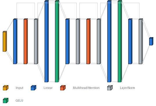
Figure 1: The model end to end. Each patch is projected to 64 numbers, two identical encoder blocks run over the 17 tokens, and the head reads position 0. The tall blue and green pairs are the feed-forward expansion inside each block; the outlines arching over are the residual connections.
Position Embeddings
Attention compares every token with every other and takes a weighted sum. Nothing in that calculation refers to where a token is, so shuffling the tokens gives the same outputs in a different order. Without something to break that symmetry a Vision Transformer sees a bag of patches rather than a picture.
Deleting them measures what they were worth.
Show the code
_, without_positions =zip(*(train(use_positions=False, seed=s) for s in SEEDS))def summarise(runs): last = [run[-1] for run in runs]returnf"{np.mean(last):.4f} ({min(last):.4f}-{max(last):.4f})", np.mean(last)with_text, with_mean = summarise(with_positions)without_text, without_mean = summarise(without_positions)print(f"{'':>28}{'mean (min-max) over '+str(len(SEEDS)) +' seeds':>26}")print(f"{'with position embeddings':>28}{with_text:>26}")print(f"{'without':>28}{without_text:>26}")print(f"{'difference':>28}{with_mean - without_mean:>+26.4f}")
                             mean (min-max) over 3 seeds
    with position embeddings     0.9828 (0.9819-0.9845)
                     without     0.8742 (0.8692-0.8799)
                  difference                    +0.1087
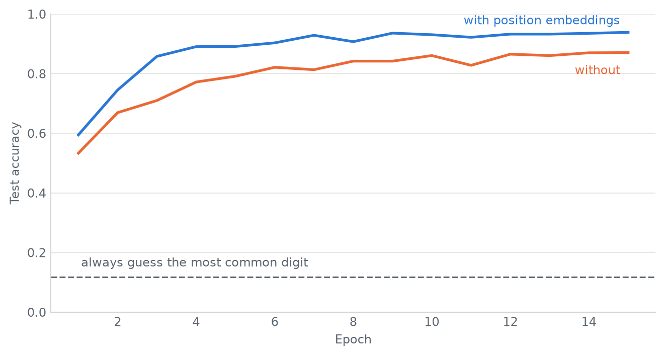
Removing them costs seven and a half points of accuracy, and the model still gets 86% of digits right without them. The gap is larger than the spread between seeds, which is what makes it worth reporting at all.
Plotted against each other, each line the mean of the three runs with the band showing their spread, and the majority-class baseline underneath:
Show the code
# Early stopping means the seeds stop at different epochs, so the band covers the# epochs every run reached rather than being padded out to the longest.shortest =min(len(run) for runs in (with_positions, without_positions) for run in runs)epochs =range(1, shortest +1)fig, ax = figure(height=3.8)ax.axhline(baseline, color=MUTED, linewidth=1.2, linestyle="--")for runs, colour, label, offset in ((with_positions, COLOURS[0], "with position embeddings", 6), (without_positions, COLOURS[1], "without", -16)): grid = np.array([run[:shortest] for run in runs]) ax.fill_between(epochs, grid.min(0), grid.max(0), color=colour, alpha=0.18, linewidth=0) ax.plot(epochs, grid.mean(0), color=colour, linewidth=2) ax.annotate(label, xy=(epochs[-1], grid.mean(0)[-1]), xytext=(-6, offset), textcoords="offset points", ha="right", fontsize=9, color=colour)ax.annotate("always guess the most common digit", xy=(1, baseline), xytext=(2, 8), textcoords="offset points", fontsize=9, color=MUTED)ax.set_ylim(0, 1.0)style_axes(ax, "Epoch", "Test accuracy")fig.tight_layout()
Figure 2: The same model with and without position embeddings. A bag of patches still says a lot about which digit it is; the layout is worth the rest.
It still works without them, which surprised me until I thought about what a bag of 7×7 patches contains. A 0 and a 1 are made of visibly different pieces however you shuffle them. Position buys the distinctions that depend on layout.
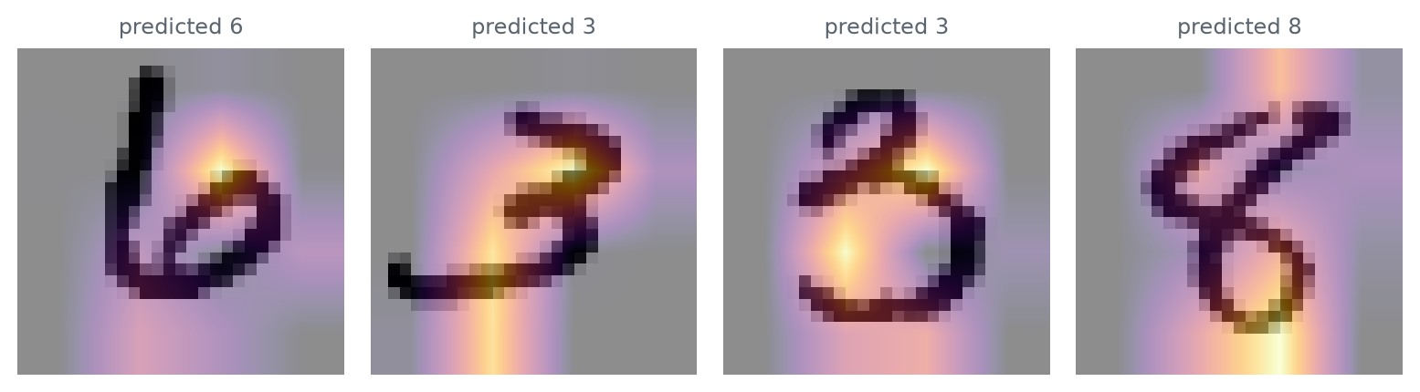
Since the classifier reads only the [CLS] token, the attention out of that position says which patches the answer actually rests on.
Figure 3: Attention from the [CLS] token in the final block. Nothing in the loss says to look at the strokes.
Conclusion
A small convolutional network beats this at MNIST scale, and Dosovitskiy et al. put transformers ahead of convolutions only with a lot of data behind them.
What this gives you:
Why it is called a transformer: it rewrites each token’s meaning using context
Why attention divides by the square root of the width
An image is a sequence of vectors, the same as a sentence
The front end is swappable, and the model behind it does not change
Captioning takes that last point literally and bolts a vision model to a language model.
The full project, with the blocks written from scratch, is on GitHub.