Early vs Late Fusion: The Gap Closes as the Model Grows

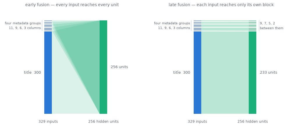
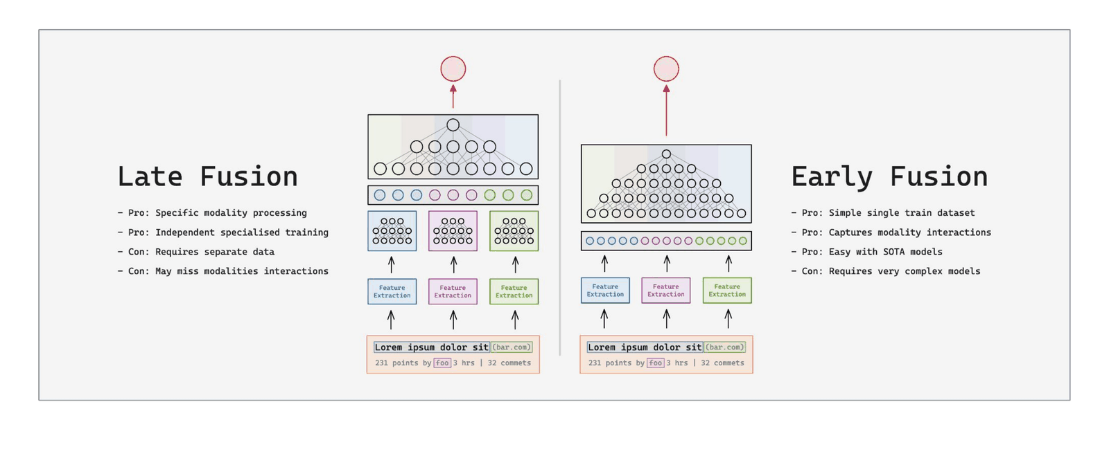
Early and late fusion are usually argued as two architectures. They are one architecture with a dial, and most of the difference is about width.

The setup is a model whose inputs come in groups: a title, a timestamp, a domain, an author. Early fusion concatenates them and runs one network over the lot. Late fusion gives each group its own network, reduces each to a score, and adds the scores. The literature [1] treats these as two designs with different strengths.

Two bits of vocabulary first, since they appear throughout.

• Spearman is a rank correlation. It asks whether two orderings agree and ignores the actual values.
• A permutation test checks whether a difference is real. Shuffle the labels between the two groups a few thousand times, and see how often chance alone produces a gap this large.

Every number below is recomputed from the raw per-seed measurements when this page is run, permutation tests included, so nothing here is a statistic I wrote down once and carried forward.

The next section is the exception. Its fusion-point curve and its width table come from a 490-run sweep that is far too large to re-run here, so those arrive as a saved image and a written-out table. Everything else, including the architecture diagram beneath this, is computed here.

# Setup, inlined rather than imported so this notebook runs on its own.
# Keep it folded; nothing below it depends on anything outside this file.

import matplotlib.pyplot as plt

# --- chart styling -------------------------------------------------------
# Categorical slots of a CVD-validated palette: blue, orange, aqua, purple.
COLOURS = ["#2a78d6", "#eb6834", "#1baf7a", "#8a63d2"]
MUTED, GRID, AXIS = "#5b6570", "#e6e6e3", "#d5d5d1"


def style_axes(ax, xlabel=None, ylabel=None, grid="y"):
    """Strip an axes back to the ink that carries information."""
    if xlabel:
        ax.set_xlabel(xlabel, color=MUTED, fontsize=9)
    if ylabel:
        ax.set_ylabel(ylabel, color=MUTED, fontsize=9)
    if grid:
        ax.grid(axis=grid, color=GRID, linewidth=0.8)
        ax.set_axisbelow(True)
    for side in ("top", "right"):
        ax.spines[side].set_visible(False)
    for side in ("left", "bottom"):
        ax.spines[side].set_color(AXIS)
    ax.tick_params(colors=MUTED, labelsize=9, length=0)
    return ax


def figure(width=7.0, height=4.2, **kw):
    fig, ax = plt.subplots(figsize=(width, height), **kw)
    return fig, ax

# --- the content-scoring first layer, drawn to scale ----------------------
# Late fusion splits the layer in proportion to how many columns each group
# brings, so the title takes 233 of 256 units and the author's three scalars get
# 2. A grid of equal cells hides exactly that, which is why this is drawn.
FUSION_GROUPS = [("title", 300, 233), ("title shape", 11, 9), ("where it links", 9, 7),
                 ("when posted", 6, 5), ("author history", 3, 2)]
_IN_X, _IN_W, _HID_X, _HID_W = 0.30, 0.055, 0.70, 0.055
_TOP, _BOTTOM, _GAP = 0.90, 0.12, 0.006


def _stack(ax, values, total, x, width, colours):
    span = (_TOP - _BOTTOM) - _GAP * (len(values) - 1)
    y, out = _BOTTOM, []
    for value, colour in zip(values, colours):
        height = span * value / total
        ax.add_patch(plt.Rectangle((x, y), width, height, facecolor=colour,
                                   edgecolor="none"))
        out.append((y, height))
        y += height + _GAP
    return out


def _wedge(ax, a, b, alpha):
    (y0, h0), (y1, h1) = a, b
    ax.fill([_IN_X + _IN_W, _IN_X + _IN_W, _HID_X, _HID_X],
            [y0, y0 + h0, y1 + h1, y1], color=COLOURS[2], alpha=alpha, lw=0, zorder=0)


def _bracket(ax, x, low, high, label, align):
    ax.plot([x] * 2, [low, high], color="#c3ccd6", linewidth=1)
    ax.text(x + (-0.007 if align == "right" else 0.007), (low + high) / 2, label,
            va="center", ha=align, fontsize=8, color=MUTED, linespacing=1.4)


def fusion_layer(ax, kind, title):
    """One panel: the 329 inputs, and the 256 hidden units they may reach."""
    ax.set_xlim(0, 1)
    ax.set_ylim(0, 1)
    ax.axis("off")
    ax.set_title(title, fontsize=10, color=MUTED, pad=6)

    inputs = _stack(ax, [g[1] for g in FUSION_GROUPS], 329, _IN_X, _IN_W,
                    [COLOURS[0]] + ["#9fb6cf"] * 4)
    if kind == "early":
        hidden = _stack(ax, [256], 256, _HID_X, _HID_W, [COLOURS[2]])
        for group in inputs:
            _wedge(ax, group, hidden[0], 0.16)
        ax.text(_HID_X + _HID_W + 0.025, hidden[0][0] + hidden[0][1] / 2, "256 units",
                va="center", fontsize=9, color=MUTED)
    else:
        hidden = _stack(ax, [g[2] for g in FUSION_GROUPS], 256, _HID_X, _HID_W,
                        [COLOURS[2]] + ["#9ed4bd"] * 4)
        for group, block_ in zip(inputs, hidden):
            _wedge(ax, group, block_, 0.30)
        ax.text(_HID_X + _HID_W + 0.025, hidden[0][0] + hidden[0][1] / 2, "233 units",
                va="center", fontsize=9, color=MUTED)
        _bracket(ax, _HID_X + _HID_W + 0.018, hidden[1][0],
                 hidden[-1][0] + hidden[-1][1], "9, 7, 5, 2\nbetween them", "left")

    ax.text(_IN_X - 0.025, inputs[0][0] + inputs[0][1] / 2, "title  300",
            va="center", ha="right", fontsize=9, color=MUTED)
    _bracket(ax, _IN_X - 0.018, inputs[1][0], inputs[-1][0] + inputs[-1][1],
             "four metadata groups\n11, 9, 6, 3 columns", "right")
    ax.text(_IN_X + _IN_W / 2, 0.045, "329 inputs", fontsize=8.5, color=MUTED,
            ha="center")
    ax.text(_HID_X + _HID_W / 2, 0.045, "256 hidden units", fontsize=8.5, color=MUTED,
            ha="center")


import json

import numpy as np

from huggingface_hub import hf_hub_download

REVISION = "f7f04575591e5dfb4996534911c0c55e993f3899"

def results(name):
    """The raw per-seed measurements, pinned to a dataset commit."""
    return json.load(open(hf_hub_download("roshbeed/ai-residency-blog-data",
                                          f"fusion/{name}.json",
                                          repo_type="dataset", revision=REVISION)))

synthetic = results("synthetic-alpha")
counts = results("pairings-counts")
logged = results("pairings-log")
ranked = results("pairings-rank")
replicate = results("pairings-replicate")
robust_128 = results("robustness-128")
robust_512 = results("robustness-512")

print(f"synthetic sweep: {len(synthetic)} interaction strengths x "
      f"{len(next(iter(synthetic.values())))} model variants")
print(f"Hacker News: {len(counts)} pairings of input groups, 10 seeds each,")
print(f"  measured on raw counts, on log1p(counts) and on rank")

synthetic sweep: 12 interaction strengths x 12 model variants
Hacker News: 11 pairings of input groups, 10 seeds each,
  measured on raw counts, on log1p(counts) and on rank

Those two sets of runs are what every number below comes out of: one where I set the answer, and one where Hacker News does.

One Architecture, Not Two

Take one hidden layer over all the inputs concatenated. Early fusion lets every hidden unit read every input. Late fusion splits the units into per-group blocks, so each block reads only its own group. It is the same layer with the off-diagonal blocks held at zero.

import matplotlib.pyplot as plt

fig, axes = plt.subplots(1, 2, figsize=(10.4, 4.6))
fusion_layer(axes[0], "early", "early fusion — every input reaches every unit")
fusion_layer(axes[1], "late", "late fusion — each input reaches only its own block")
fig.tight_layout()

Figure 1: The first layer of each architecture, drawn to scale. Late fusion splits the 256 units in proportion to how many columns each group brings, so the title takes 233 of them and the other four share 23. Everything after this layer is identical in both.

So early and late are two ends of one dial: which layer do the groups first meet at? Everything before it is block-diagonal, everything from it on is shared. Fusing at layer 1 is early fusion, fusing at the last layer is late fusion, and the question stops being which is better. It becomes: how long can you delay fusion before it costs you?

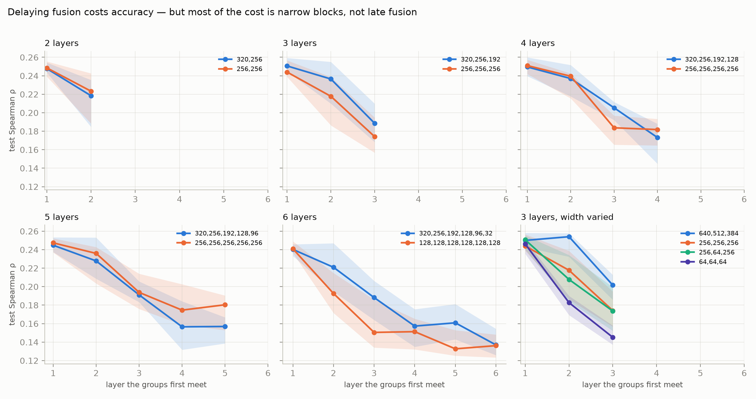
I swept that across 13 layer shapes at every valid fusion point, ten seeds each, 490 runs. Ten rather than three because late fusion’s three-seed spread was 0.106 Spearman against early fusion’s 0.026, wide enough to swallow the effect being measured.

Delaying always costs something, and almost all of that cost is how wide the isolated layer is rather than the delay itself. At depth three, holding everything else fixed and changing only the width:

shape	first-layer width	fuse at 1	fuse at 2	cost of one private layer
640,512,384	640	0.249	0.254	+0.005
320,256,192	320	0.251	0.242	−0.008
256,256,256	256	0.243	0.191	−0.053
64,64,64	64	0.247	0.186	−0.061

At 640 units a private layer per group is free. At 64 it costs 0.061, more than the entire early-versus-late gap. The reason is the allocation rule. Each group’s share of a layer is proportional to how many columns it brings. The author’s history gets round(w × 3/329) units: six at width 640, and one at width 64.

A narrow block-diagonal layer does not delay fusion so much as strangle four of the five inputs before they reach it.

A Control With a Known Answer

Before trusting any of this on real data, the measurement needs checking. So here is a target whose interaction strength I set myself:

\[y = g + h + \alpha \cdot g h\]

At \(\alpha = 0\) the two groups contribute independently and late fusion is exactly the right model. As \(\alpha\) rises, a model that can only add should fall behind.

This is a real sweep: twelve interaction strengths, three architectures, four widths, ten seeds each.

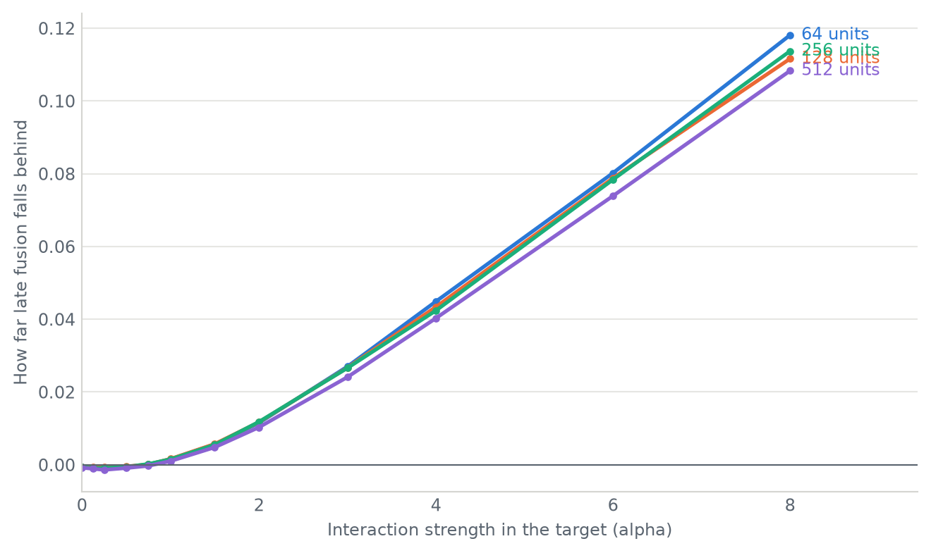
alphas = sorted(synthetic, key=float)
widths = [64, 128, 256, 512]

fig, ax = figure(height=4.2)
for width, colour in zip(widths, COLOURS):
    gap = [synthetic[a][f"early@{width}"]["median"] - synthetic[a][f"late-snoek@{width}"]["median"]
           for a in alphas]
    ax.plot([float(a) for a in alphas], gap, color=colour, linewidth=2, marker="o", markersize=3)
    ax.annotate(f"{width} units", xy=(float(alphas[-1]), gap[-1]), xytext=(6, 0),
                textcoords="offset points", fontsize=9, color=colour, va="center")

ax.axhline(0, color=MUTED, linewidth=0.8)
ax.set_xlim(0, float(alphas[-1]) * 1.18)
style_axes(ax, "Interaction strength in the target (alpha)", "How far late fusion falls behind")
fig.tight_layout()

Figure 2: Snoek late fusion against early fusion on a target with a known interaction, at four widths. The penalty grows with the interaction and barely moves with width.

The gap at the strongest interaction, at each width:

widest, narrowest = "512", "64"
worst = alphas[-1]
print(f"at alpha={worst}:")
for width in widths:
    gap = (synthetic[worst][f"early@{width}"]["median"]
           - synthetic[worst][f"late-snoek@{width}"]["median"])
    print(f"  {width:>4} units: late fusion is {gap:.3f} behind")

zero_gap = max(abs(synthetic["0.0"][f"early@{w}"]["median"]
                   - synthetic["0.0"][f"late-snoek@{w}"]["median"]) for w in widths)
print(f"\nat alpha=0, the largest gap at any width is {zero_gap:.4f}")

at alpha=8.0:
    64 units: late fusion is 0.118 behind
   128 units: late fusion is 0.112 behind
   256 units: late fusion is 0.114 behind
   512 units: late fusion is 0.108 behind

at alpha=0, the largest gap at any width is 0.0008

Two things to take from that.

The measurement works. When an interaction exists this comparison finds it, and when one doesn’t the two architectures land within 0.001 of each other at every width. So a null result later is a null result rather than a broken harness.

Width barely rescues it. Eight times the hidden units recovers about 9% of the gap, the opposite of what the width sweep showed on real data. The difference matters. When an interaction really exists in the target, an additive model cannot buy its way out with capacity. It’s not underfitting. It’s the wrong shape.

The Real Data

The same comparison on real Hacker News upvote counts, for every pairing of input groups. One model cannot represent an interaction: a tower each, reduced to one score, then summed. The other can.

The control that decides whether this means anything is capacity. A joint model has more parameters, so it can win for reasons that have nothing to do with interaction. So the additive model here gets towers three times wider: still structurally unable to represent an interaction, and now with more parameters than its rival. Anything the joint model wins by is the interaction, not the budget.

def permutation_test(a, b, trials=20_000, seed=0):
    """How often would shuffling the labels produce a difference this large?"""
    a, b = np.asarray(a), np.asarray(b)
    observed = np.median(b) - np.median(a)
    pool = np.concatenate([a, b])
    rng = np.random.default_rng(seed)

    hits = 0
    for _ in range(trials):
        rng.shuffle(pool)
        if abs(np.median(pool[len(a):]) - np.median(pool[:len(a)])) >= abs(observed):
            hits += 1
    return observed, (hits + 1) / (trials + 1)

def interaction(dataset, pairing):
    return permutation_test(dataset[pairing]["additive-matched"], dataset[pairing]["joint"])

rows = sorted(((name, *interaction(counts, name)) for name in counts), key=lambda r: -r[1])

print(f"{'does the first group depend on the second?':<42} {'effect':>9} {'p':>8}")
for name, effect, p in rows:
    print(f"{name:<42} {effect:>+9.4f} {p:>8.3f}{'*' if p < 0.05 else ' '}")

does the first group depend on the second?    effect        p
title x when you post                        +0.0381    0.000*
title x all metadata                         +0.0220    0.001*
title x title shape                          +0.0090    0.007*
title x where it links                       +0.0081    0.139 
title x the author                           +0.0020    0.628 
where x author                               +0.0013    0.307 
author x title shape                         -0.0008    0.721 
when x title shape                           -0.0014    0.619 
where x title shape                          -0.0062    0.065 
when x author                                -0.0067    0.066 
when x where                                 -0.0117    0.023*

One row is far larger than the rest, three clear the significance test in the same direction, and seven of the eleven rows sit on zero.

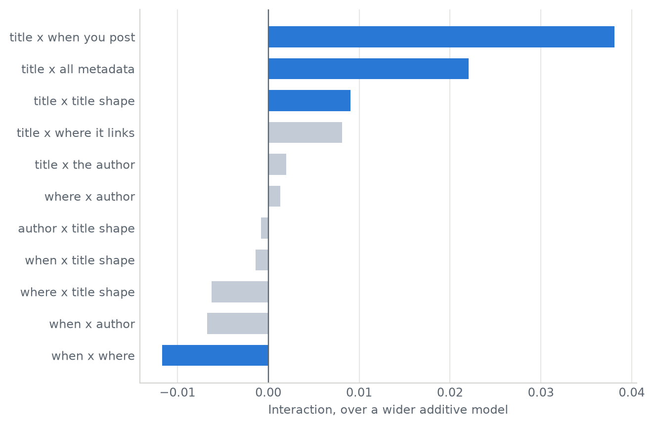
Drawn as a chart, sorted by effect:

names = [r[0] for r in rows][::-1]
effects = [r[1] for r in rows][::-1]
significant = [r[2] < 0.05 for r in rows][::-1]

fig, ax = figure(height=4.6)
ax.barh(range(len(names)), effects,
        color=[COLOURS[0] if s else "#c3ccd6" for s in significant], height=0.66)
ax.axvline(0, color=MUTED, linewidth=0.9)
ax.set_yticks(range(len(names)), names, fontsize=9)
style_axes(ax, "Interaction, over a wider additive model", grid="x")
fig.tight_layout()

Figure 3: Each pairing’s interaction against the capacity-matched additive control. Filled bars survive a permutation test at p < 0.05.

The title and the timing is the largest effect in the table by a distance, and it decided the architecture this service serves. The mechanism is the one in the other post. A good title doesn’t add a fixed number of upvotes. It multiplies whatever the timing was going to give you, and a model that scores the two separately and sums them can only add.

Notice how much of the rest of the table is noise. Two-thirds of the pairings are indistinguishable from zero and five point the wrong way. This is one specific pair of inputs interacting, not a general property of the task.

Units Matter

Additivity is not a property of data. It is a property of the units you measure the data in.

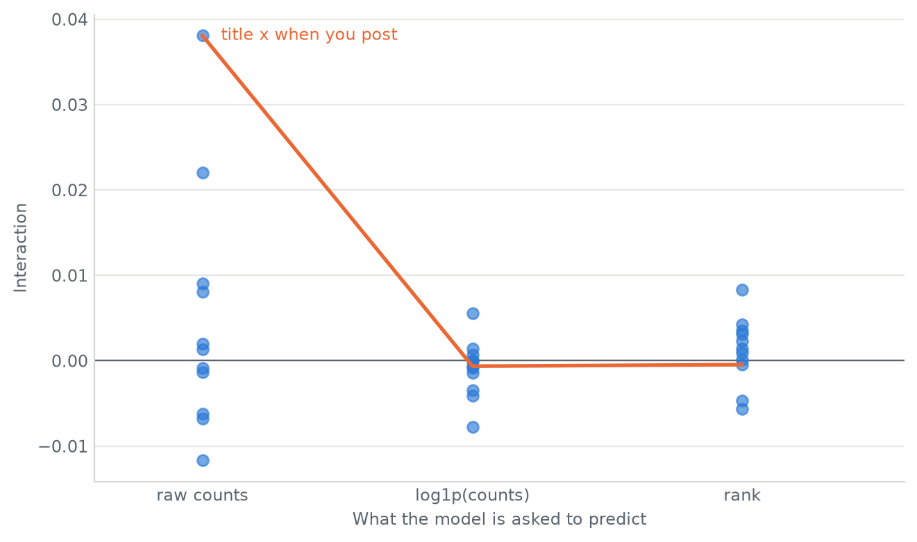
So I ran the identical comparison three times. Same models, same seeds, same everything. Once against the raw count, once against log1p(score), once against rank.

targets = [("raw counts", counts), ("log1p(counts)", logged), ("rank", ranked)]

fig, ax = figure(height=4.2)
for x, (label, dataset) in enumerate(targets):
    values = [np.median(dataset[n]["joint"]) - np.median(dataset[n]["additive-matched"])
              for n in dataset]
    ax.scatter([x] * len(values), values, s=36, color=COLOURS[0], alpha=0.65, zorder=3)

highlight = "title x when you post"
ax.plot(range(3), [np.median(d[highlight]["joint"]) - np.median(d[highlight]["additive-matched"])
                   for _, d in targets], color=COLOURS[1], linewidth=2, zorder=4)
ax.annotate(highlight, xy=(0, np.median(counts[highlight]["joint"])
                           - np.median(counts[highlight]["additive-matched"])),
            xytext=(10, 0), textcoords="offset points", fontsize=9,
            color=COLOURS[1], va="center")

ax.axhline(0, color=MUTED, linewidth=0.9)
ax.set_xlim(-0.4, 2.6)
ax.set_xticks(range(3), [t[0] for t in targets])
style_axes(ax, "What the model is asked to predict", "Interaction")
fig.tight_layout()

Figure 4: The same eleven comparisons in three coordinate systems. The interaction is a property of the raw counts and survives neither transformation.

Listing which cells survive a permutation test in each coordinate system makes the difference concrete:

for label, dataset in targets:
    print(f"{label}:")
    for name in dataset:
        effect, p = interaction(dataset, name)
        if p < 0.05:
            print(f"    {name:<26} {effect:>+8.4f}   p={p:.3f}")
    print()

raw counts:
    title x when you post       +0.0381   p=0.000
    title x title shape         +0.0090   p=0.007
    title x all metadata        +0.0220   p=0.001
    when x where                -0.0117   p=0.023

log1p(counts):
    title x the author          -0.0041   p=0.019
    when x author               -0.0077   p=0.001
    author x title shape        +0.0055   p=0.001

rank:
    title x where it links      +0.0035   p=0.013
    title x title shape         +0.0042   p=0.007
    where x title shape         +0.0014   p=0.035
    author x title shape        +0.0083   p=0.001

The big one is gone. title x when you post goes from +0.0381 to roughly zero under both transformations, and the cells that remain significant are different ones, an order of magnitude smaller.

A logarithm turns multiplication into addition, so an additive model fitted on log1p can represent precisely the thing it couldn’t represent on counts. Rank keeps every comparison between posts and discards all the magnitudes, and the interaction goes with them.

So this interaction lives in how large the counts get, not in which post beats which. A service that ranked posts wouldn’t need early fusion at all. This one predicts counts, so it does.

One pairing runs the other way, and it’s the interesting one. author x title shape is the mirror image of title x when you post. On raw counts it is nothing at all: the wrong sign, and nowhere near significant. It appears only once the counts have been transformed away, and in both log1p and rank it is the strongest cell that survives.

So that one is an interaction in ordering rather than in magnitude. A known name’s Show HN: really does land differently from a stranger’s. It changes who beats whom, and not by how much.

Two pairings, then, and neither of them is visible in the other’s coordinate system. I find this the most useful thing in the project, because it generalises well past fusion. “Is there an interaction in my data” isn’t a well-formed question until you have said what scale you’re measuring on.

A caveat over all three tables. Eleven pairings in three coordinate systems is thirty-three tests at p < 0.05, and one or two hits at that threshold is what chance alone hands you. None of this is corrected for that. The readings worth defending are the ones that are far larger than everything else in their table and come back on a second independent run; the cells sitting at p ≈ 0.02 are worth a shrug and no more.

It also replicates, which matters given how many times I had to withdraw a reading of this comparison.

print(f"{'pairing':<26} {'first run':>10} {'replication':>12}")
for name in ("title x when you post", "title x all metadata", "title x title shape"):
    first = np.median(counts[name]["joint"]) - np.median(counts[name]["additive-matched"])
    again = np.median(replicate[name]["joint"]) - np.median(replicate[name]["additive-matched"])
    print(f"{name:<26} {first:>+10.4f} {again:>+12.4f}")

pairing                     first run  replication
title x when you post         +0.0381      +0.0334
title x all metadata          +0.0220      +0.0222
title x title shape           +0.0090      +0.0134

Same three cells, same signs, similar sizes on a second independent run. The one that matters moves from +0.0381 to +0.0334 and stays the largest.

Late Fusion’s Advantage

The surveys don’t mainly claim late fusion is more accurate. They claim it’s more robust: when one input goes missing or bad, it can lean on the surviving branch, where early fusion has entangled everything in its first layer.

They are right, and it is measurable. Train all three architectures on clean data, then damage one input only at inference.

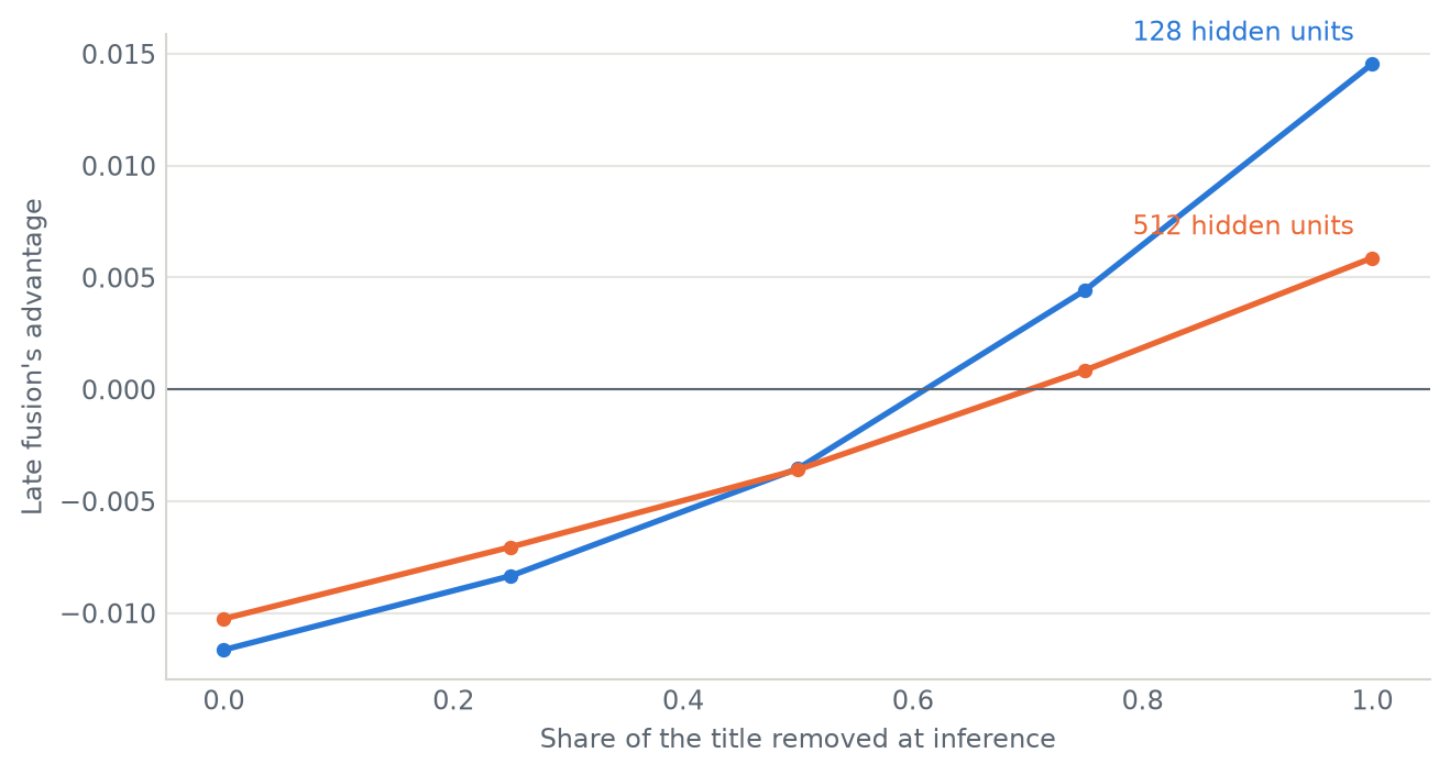
damage = ["0.0", "0.25", "0.5", "0.75", "1.0"]

fig, ax = figure(height=3.8)
for data, colour, label in ((robust_128, COLOURS[0], "128 hidden units"),
                            (robust_512, COLOURS[1], "512 hidden units")):
    advantage = [np.median(data[f"missing-title@{d}"]["late-snoek"])
                 - np.median(data[f"missing-title@{d}"]["early"]) for d in damage]
    ax.plot([float(d) for d in damage], advantage, color=colour, linewidth=2, marker="o",
            markersize=4)
    ax.annotate(label, xy=(1.0, advantage[-1]), xytext=(-6, 8), textcoords="offset points",
                ha="right", fontsize=9, color=colour)

ax.axhline(0, color=MUTED, linewidth=0.8)
style_axes(ax, "Share of the title removed at inference", "Late fusion's advantage")
fig.tight_layout()

Figure 5: Late fusion’s advantage when an input is damaged, at two widths. It is real at 128 hidden units and much smaller at 512.

Putting numbers on the two ends of that:

for data, label in ((robust_128, "128 units"), (robust_512, "512 units")):
    clean = (np.median(data["missing-title@0.0"]["late-snoek"])
             - np.median(data["missing-title@0.0"]["early"]))
    broken = (np.median(data["missing-title@1.0"]["late-snoek"])
              - np.median(data["missing-title@1.0"]["early"]))
    print(f"{label}: late fusion pays {-clean:+.3f} when nothing is wrong "
          f"to gain {broken:+.3f} when the title is gone")

128 units: late fusion pays +0.012 when nothing is wrong to gain +0.015 when the title is gone
512 units: late fusion pays +0.010 when nothing is wrong to gain +0.006 when the title is gone

So the insurance is real. It’s also a small-model effect.

At 128 hidden units late fusion gives up 0.012 on clean data and gains 0.015 when the title disappears, so the cover roughly pays for itself. At 512 it gives up 0.010 and gains 0.006. Early fusion now has enough capacity to cope on its own.

Conclusion

Four separate measurements point the same way: the fusion-point sweep, the width sweep, the pairing table and the robustness probe. It is not the conclusion I expected to write.

The architectural distinction mostly matters when something else is constrained.

• Given enough width, early fusion matches late fusion’s robustness
• Given enough width, late fusion matches early fusion’s accuracy on this data. On the synthetic target it never catches up, and eight times the width buys back about 9% of the gap
• The gap is widest where the model is too small, and closes as it grows
• An interaction that exists in one coordinate system may not exist in another

So “early versus late fusion” is not a ranking. It is a question about your data and your budget. Is there an interaction to model, and can you afford the width to model it? Quote a fusion result without the width it was measured at and you have not said anything.

The measurements, and the service they came from, are on GitHub.

---

[1] Snoek, Worring, Smeulders. Early versus Late Fusion in Semantic Video Analysis. ACM Multimedia 2005.