Predicting Hacker News Upvotes

The second half of week 1. Four kinds of input, one number to predict, and a question about where in the model the inputs should be combined.

The second project of week 1, and it’s the first one’s motivating example with a real dataset behind it.

The word2vec post started here. Predict a number about someone from a few things you know. Most features are easy. One is a free-text box, and there’s no obvious way to encode it.

The answer was to learn a vector per word and average them.

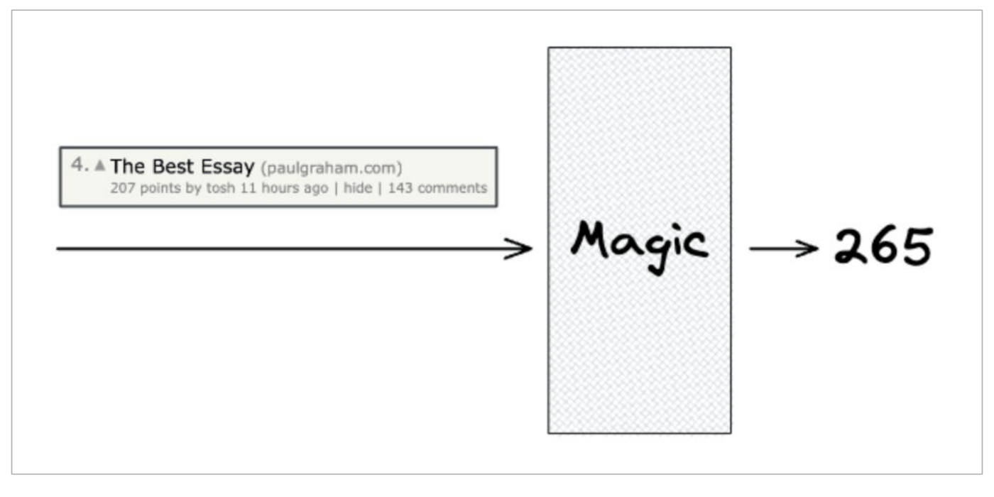
This project is that model, with Hacker News in place of the income form. Predict how many upvotes a post will get, from its title, where it links, when it was submitted and who by.

872,554 real posts from November 2023 to August 2026, split by time rather than at random. Scores drift and posts from the same day compete for the same front page, so a random split would let the model see the future of its own test set.

The Data

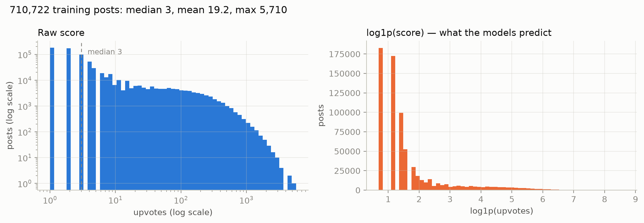
The median post scores 3. The maximum is 5,710. On a distribution this skewed the typical post and the average post are six times apart. That gap decides more than the architecture does.

One input is deliberately missing. The comment count predicts the score very well. It is also not known when a post is submitted. A model using it would score beautifully and answer a question nobody asked.

The author’s history has the same hazard, so it is built only from their earlier posts.

Early and Late Fusion

A post arrives as four different kinds of thing: some text, a timestamp, a link, an author. They have to be combined somewhere, and there are two conventional places to do it.

I built late fusion as early fusion with the cross-group weights deleted. Both models are the same stack: a first layer taking 329 inputs onto 256 hidden units, a shared 256 → 256 layer, then the head. The only difference is that late fusion’s first layer is block-diagonal, so the title cannot reach the hidden units the timestamp owns.

The shared second layer is there on purpose. Without it, late fusion would have no trunk at all after the join. The two models would then differ in depth as well as in connectivity. That gives you two explanations for any gap instead of one.

architecture	first layer	then	parameters
metadata only	29 → 256	256 → 256 → 1	73,793
title only	300 → 256	256 → 256 → 1	143,169
early fusion	329 → 256 dense	256 → 256 → 1	150,593
late fusion	300→233 \| 6→5 \| 9→7 \| 11→9 \| 3→2	256 → 256 → 1	136,467

Look at that last row. Hidden units are split in proportion to how many columns each group brings, so the 300-dimensional title owns 233 of the 256 and the author’s three scalars get 2. That keeps the first layer the same shape in both models, which is what makes the comparison a comparison. It also quietly throttles four of the five inputs, and that becomes the whole story later.

Results

Held-out June to August 2026: 69,275 posts carrying 1,309,690 upvotes, each row the mean of three seeds.

model	median error	mean predicted	highest prediction	share of upvotes
what actually happened	—	18.9	3,158	100%
guess the average every time	16.2	19.2	19	101%
TF-IDF + Ridge on the title	13.0	21.4	453	113%
title only	11.1	15.7	529	83%
metadata only	13.2	18.7	512	99%
early fusion (served)	10.1	17.0	1,226	90%
late fusion	10.1	15.8	825	84%

A median error of 10.1 against 16.2 for guessing the average is real work.

The column I care about more is the highest prediction. The served model will say 1,226 for the right post. It can call a front-page hit, and those are the posts anyone actually cares about.

Neither input alone is a good model. Title only lands at 11.1 and metadata only at 13.2, against 10.1 for the two together.

Which Inputs Matter

Zero one input at a time and see what the prediction loses:

input removed	effect
the title	−0.11
the author’s history	−0.07
when it was posted	−0.03
the title’s shape	−0.02
where it links	+0.02

The title carries the most and the author’s history is second, which I expected. The domain is the surprise: removing it slightly improves the model. At this width it is costing more in capacity than it returns in signal.

This has to be measured on early fusion. On the block-diagonal model the title owns 233 of the 256 hidden units, so an ablation there reports the allocation rule as much as it reports the signal.

Why the Architecture Question Dissolved

At 256 hidden units early fusion wins: ρ 0.2487 against late’s 0.2291 over 40 and 30 seeds, a gap of 0.020 that separates cleanly at p < 0.001. That is a solid number rather than the three-seed coincidence it started life as.

It is also a statement about 256 hidden units and not about fusion. Run the same comparison at matched capacity from 128 to 2048 units and the gap only exists at the smallest budget. From 256 up the two are indistinguishable, because what was being measured was the throttling in that allocation table, not the connectivity.

The mechanism is easy to see on a target where I control the answer. Two groups of inputs, and a target that is their sum plus a product term I can turn up:

\[y = s_A + s_B + \alpha \cdot s_A s_B\]

At α = 0 a model that scores the groups separately and adds is exactly right. As α rises it has nothing left to represent the product with.

The code below builds both architectures from one class, changing only which first-layer weights are allowed to be non-zero, and fits each at six values of α.

import sys

sys.path.insert(0, "..")
import numpy as np
import torch
import torch.nn as nn
from _style import COLOURS, MUTED, figure, style_axes

D, H, N = 6, 64, 6000


def mask_for(kind):
    """Which first-layer weights are allowed to be non-zero."""
    mask = torch.ones(2 * D, H)
    if kind == "late":
        mask[:D, H // 2:] = 0
        mask[D:, :H // 2] = 0
    return mask


def make_data(alpha, seed):
    g = torch.Generator().manual_seed(seed)
    a, b = torch.randn(N, D, generator=g), torch.randn(N, D, generator=g)
    wa = torch.randn(D, generator=g) / D**0.5
    wb = torch.randn(D, generator=g) / D**0.5
    score_a, score_b = a @ wa, b @ wb
    y = score_a + score_b + alpha * score_a * score_b
    return torch.cat([a, b], 1), (y - y.mean()) / y.std()


class Fusion(nn.Module):
    """One architecture. `kind` only decides which weights may be non-zero."""

    def __init__(self, kind, seed):
        super().__init__()
        torch.manual_seed(seed)
        self.first, self.head = nn.Linear(2 * D, H), nn.Linear(H, 1)
        self.register_buffer("mask", mask_for(kind))

    def forward(self, x):
        hidden = torch.relu(x @ (self.first.weight.T * self.mask) + self.first.bias)
        return self.head(hidden).squeeze(-1)


def variance_explained(kind, alpha, seed, steps=1500):
    X, y = make_data(alpha, seed)
    split = int(0.7 * N)
    model = Fusion(kind, 100 + seed)
    optimiser = torch.optim.Adam(model.parameters(), lr=0.02)
    for _ in range(steps):
        loss = ((model(X[:split]) - y[:split]) ** 2).mean()
        optimiser.zero_grad()
        loss.backward()
        optimiser.step()
    with torch.no_grad():
        return 1 - ((model(X[split:]) - y[split:]) ** 2).mean().item() / y[split:].var().item()


alphas = [0.0, 0.25, 0.5, 1.0, 2.0, 4.0]
early = [np.median([variance_explained("early", a, s) for s in range(3)]) for a in alphas]
late = [np.median([variance_explained("late", a, s) for s in range(3)]) for a in alphas]

print(f"{'alpha':>6} {'early':>8} {'late':>8} {'gap':>8}")
for a, e, l in zip(alphas, early, late):
    print(f"{a:>6} {e:>8.4f} {l:>8.4f} {e - l:>+8.4f}")

 alpha    early     late      gap
   0.0   1.0000   1.0000  -0.0000
  0.25   0.9999   0.9505  +0.0494
   0.5   0.9998   0.8236  +0.1762
   1.0   0.9997   0.5135  +0.4861
   2.0   0.9991   0.1224  +0.8766
   4.0   0.9996  -0.0922  +1.0918

Both architectures are the same network, drawn once.

from _arch import diagram

diagram(Fusion("early", 0), input_shape=(1, 2 * D), style="flow")

Figure 1: One architecture, drawn once. Early and late fusion are this same network. The only difference is which of the first layer’s weights are allowed to be non-zero.

Plotting the sweep shows where the two architectures separate.

fig, ax = figure(height=3.8)
ax.plot(alphas, early, color=COLOURS[0], linewidth=2, marker="o", markersize=4)
ax.plot(alphas, late, color=COLOURS[1], linewidth=2, marker="o", markersize=4)
ax.annotate("early fusion", xy=(alphas[-2], early[-2]), xytext=(0, 10),
            textcoords="offset points", fontsize=9, color=COLOURS[0], ha="center")
ax.annotate("late fusion", xy=(alphas[-2], late[-2]), xytext=(0, -18),
            textcoords="offset points", fontsize=9, color=COLOURS[1], ha="center")
ax.axhline(0, color=MUTED, linewidth=0.8)
style_axes(ax, "Interaction strength (alpha)", "Held-out R-squared")
fig.tight_layout()

Figure 2: Held-out R-squared as the product term grows. With no interaction the two architectures are identical.

At α = 0 the two are indistinguishable. Deleting the cross-group weights costs nothing when there’s nothing across the groups to model. Everything after that is the product term, and late fusion cannot represent it at any width.

So the useful question is whether Hacker News has one.

It does, in one place: the title and the timing. Fitted on the raw upvote counts, against an additive control given towers three times wider so it has more parameters, that pairing is worth +0.038 and is the largest effect in the table.

A good title doesn’t add a fixed number of upvotes. It multiplies whatever the timing was going to give you. The same title is worth a handful of points at a dead hour and hundreds when the site is awake, and a model that scores the two separately and sums the scores can only add.

One thing took me a while to see. Fit the identical comparison on log1p(score) and the interaction disappears, because a logarithm turns multiplication into addition. Fit it on rank and it disappears too, since rank keeps every comparison between posts and throws away the magnitudes. The interaction lives in how large the counts get, not in which post beats which. A service that ranked posts would not need early fusion at all. This one predicts counts, so it does.

I go through that properly in the fusion deep dive.

The Ceiling

All of which sits under a harder limit.

A quarter of all linked posts are reposts: 85,340 URLs submitted more than once. That gives a natural experiment, because the content is held fixed and everything else varies. The two scores agree only weakly. Among URLs whose first submission scored between 2 and 5, the second submission reached a maximum of 2,645.

Knowing that identical content has already hit the front page roughly doubles the odds it will again, from 5.6% to 11.3%. That is all it buys. The content explains some of the outcome and timing, luck and whoever happened to be reading explain a lot of the rest.

There is a second ceiling, closer to home. This model averages word vectors, and averaging throws away word order, so Google acquires OpenAI and OpenAI acquires Google are the same input. A fine-tuned sentence transformer reads the difference and scores better. A deeper network on the same averaged vectors does not. The limit is the representation, not the model.

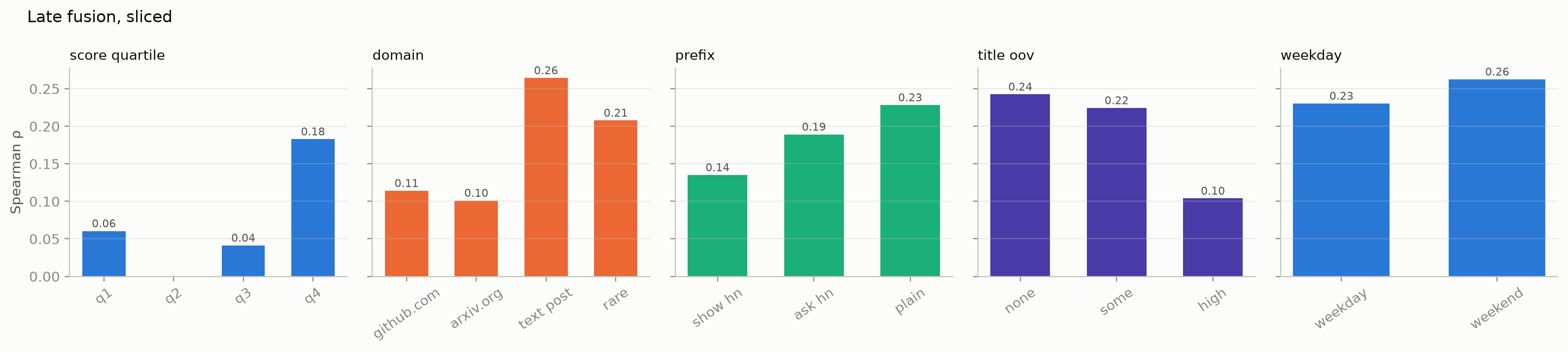
Show HN posts are the hardest slice, which makes sense: they compete on what was built rather than on how it was described, and a title carries less of that.

Conclusion

• The title carries the most signal, and the author’s history is second
• Combining inputs beats either alone
• Early fusion wins at this width, and stops winning once the model is big enough
• The interaction is in the counts, not the ordering
• Most of the outcome is luck, and no architecture fixes that

The full project is on GitHub.